探索数据分布 |设置 2
先决条件:探索数据分布 |设置 1
与探索数据分布相关的术语
-> Boxplot
-> Frequency Table
-> Histogram
-> Density Plot
要获取所使用的 csv 文件的链接,请单击此处。
加载库
Python3
import numpy as np
import pandas as pd
import seaborn as sns
import matplotlib.pyplot as plt
Python3
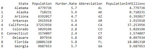
data = pd.read_csv("../data/state.csv")

# Adding a new column with derived data
data['PopulationInMillions'] = data['Population']/1000000

print (data.head(10))
Python3
# Histogram Population In Millions

fig, ax2 = plt.subplots()
fig.set_size_inches(9,  15)

ax2 = sns.distplot(data.PopulationInMillions, kde = False)
ax2.set_ylabel("Frequency", fontsize = 15)
ax2.set_xlabel("Population by State in Millions", fontsize = 15)
ax2.set_title("Population - Histogram", fontsize = 20)
Python3
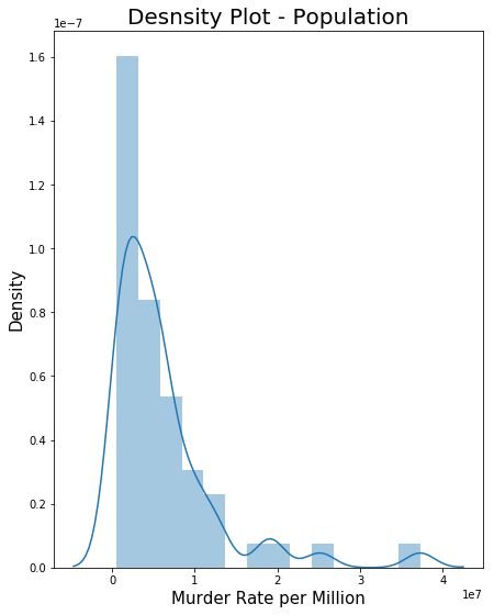
# Density Plot - Population

fig, ax3 = plt.subplots()
fig.set_size_inches(7,  9)

ax3 = sns.distplot(data.Population, kde = True)
ax3.set_ylabel("Density", fontsize = 15)
ax3.set_xlabel("Murder Rate per Million", fontsize = 15)
ax3.set_title("Density Plot - Population", fontsize = 20)
加载数据中
Python3
data = pd.read_csv("../data/state.csv")

# Adding a new column with derived data
data['PopulationInMillions'] = data['Population']/1000000

print (data.head(10))
输出 :
- 直方图:它是一种通过频率表可视化数据分布的方法,其中 x 轴上的 bin 和 y 轴上的数据计数。
代码 - 直方图
Python3
# Histogram Population In Millions

fig, ax2 = plt.subplots()
fig.set_size_inches(9,  15)

ax2 = sns.distplot(data.PopulationInMillions, kde = False)
ax2.set_ylabel("Frequency", fontsize = 15)
ax2.set_xlabel("Population by State in Millions", fontsize = 15)
ax2.set_title("Population - Histogram", fontsize = 20)
- 输出 :

- 密度图:它与直方图有关,因为它显示数据值以连续线分布。这是一个平滑的直方图版本。下面的输出是叠加在直方图上的密度图。
代码 - 数据的密度图
Python3
# Density Plot - Population

fig, ax3 = plt.subplots()
fig.set_size_inches(7,  9)

ax3 = sns.distplot(data.Population, kde = True)
ax3.set_ylabel("Density", fontsize = 15)
ax3.set_xlabel("Murder Rate per Million", fontsize = 15)
ax3.set_title("Density Plot - Population", fontsize = 20)
- 输出 :