使用 R 中的拼凑包绘制绘图组合

在本文中，我们将讨论如何使用 R 编程语言中的 patchwork 包绘制绘图组合。 patchwork 包可以更轻松地在单个图中绘制不同的 ggplots。我们将需要用于绘制数据的 ggplot2 包和用于组合不同 ggplots 的 patchwork 包。

让我们首先正常且独立地绘制所有图。

示例：在条形图中绘制数据集

R

library(ggplot2)
library(patchwork)
  
data(iris)
  
head(iris)
  
# Plotting the bar chart
gfg1 <- ggplot(iris, aes(Sepal.Length, Petal.Length, color = Species)) + 
geom_bar(stat = "identity")
  
gfg1

输出 ：

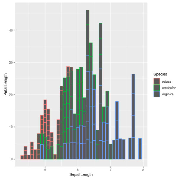
条形图

示例：在散点图中绘制数据集

电阻

library(ggplot2)
library(patchwork)
  
data(iris)
  
head(iris)
  
# Scatterplot
gfg2 <- ggplot(iris, aes(Sepal.Length, Petal.Length, 
                         color = Species)) + geom_point()
  
gfg2

输出 ：

散点图

示例：在折线图中绘制数据集

电阻

library(ggplot2)
library(patchwork)
  
data(iris)
  
head(iris)
  
# Line plot
gfg3 <- ggplot(iris, aes(Sepal.Length, Petal.Length, 
                         color = Species)) + geom_line()
  
gfg3

输出 ：

线图

现在让我们看看这三个图如何以不同的方向组合。

垂直绘图

垂直方向结合了地块，这些地块彼此并排放置。我们将采用上面的 ggplot2 图并添加它们以垂直排列它们。 +运算符用于在同一图中并排排列这些图。

示例：在同一帧中垂直排列图

电阻

library(ggplot2)
library(patchwork)
  
data(iris)
  
head(iris)
  
gfg1 <- ggplot(iris, aes(Sepal.Length, Petal.Length, 
                         color = Species)) + geom_bar(stat = "identity")
  
gfg2 <- ggplot(iris, aes(Sepal.Length, Petal.Length, 
                         color = Species)) + geom_point()
  
gfg3 <- ggplot(iris, aes(Sepal.Length, Petal.Length, 
                         color = Species)) + geom_line()
  
# Combination of plots by arranging them side by side
gfg_comb_1 <- gfg1 + gfg2 + gfg3
  
gfg_comb_1

输出 ：

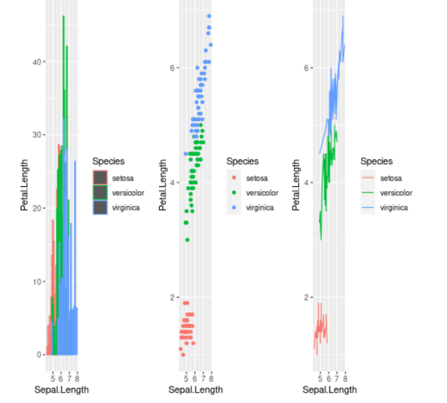
垂直方向

以不同的宽度排列

这些图的第二种组合是将它们以不同宽度排列在同一图形窗口中的多行和多列中。不同的宽度方向根据宽度将绘图排列在不同的行中。基本上，第一个图放置在第一行，其他两个图水平放置在下一行。

我们在要开始新行的位置使用斜杠(/)运算符。所以我们把它放在第一个情节之后。然后，我们使用 add (+)运算符在下一个新行上水平排列其他两个图。

示例：排列具有不同宽度的图

电阻

library(ggplot2)
library(patchwork)
  
data(iris)
  
head(iris)
  
gfg1 <- ggplot(iris, aes(Sepal.Length, Petal.Length,
                         color = Species)) + 
geom_bar(stat = "identity")
  
gfg2 <- ggplot(iris, aes(Sepal.Length, Petal.Length, 
                         color = Species)) +
geom_point()
  
gfg3 <- ggplot(iris, aes(Sepal.Length, Petal.Length, 
                         color = Species)) +
geom_line()
  
# Arranging the plots in different widths
gfg_comb_2 <- gfg1 / (gfg2 + gfg3)
  
gfg_comb_2

输出 ：

不同宽度方向

排列不同的高度

这些图的第三种组合是将它们排列在同一图形窗口中的多行和多列中的不同高度。不同的高度方向根据高度将地块排列在不同的行中。基本上，前两个图水平排列，最后一个图放置在第二个图下方。

我们使用加(+)运算符来水平排列前两个图。然后我们对第三个图使用斜线(/)运算符将其放置在第二个图下方的新行上。

示例：排列具有不同高度的地块

电阻

library(ggplot2)
library(patchwork)
  
data(iris)
  
head(iris)
  
gfg1 <- ggplot(iris, aes(Sepal.Length, Petal.Length,
                         color = Species)) + 
geom_bar(stat = "identity")
  
gfg2 <- ggplot(iris, aes(Sepal.Length, Petal.Length,
                         color = Species)) +
geom_point()
  
gfg3 <- ggplot(iris, aes(Sepal.Length, Petal.Length,
                         color = Species)) + 
geom_line()
  
# Arrangement of plots according to 
# different heights
gfg_comb_3 <- gfg1 + gfg2 / gfg3
  
gfg_comb_3

输出 ：

不同高度方向

水平绘图

图的最后组合是将它们水平排列。这些图被放置在另一个下方。我们将使用斜线 ( / )运算符将这些图放在一个新行中，一个在另一个图下方。

示例：垂直排列绘图

电阻

library(ggplot2)
library(patchwork)
  
data(iris)
  
head(iris)
  
gfg1 <- ggplot(iris, aes(Sepal.Length, Petal.Length, color = Species)) + 
geom_bar(stat = "identity")
  
gfg2 <- ggplot(iris, aes(Sepal.Length, Petal.Length, color = Species)) + 
geom_point()
  
gfg3 <- ggplot(iris, aes(Sepal.Length, Petal.Length, color = Species)) + 
geom_line()
  
# Combination of plots by arranging them 
# horizontally
gfg_comb_4 <- gfg1 / gfg2 / gfg3
  
gfg_comb_4

输出 ：

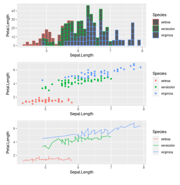
水平方向