在 MATLAB 中使用一阶导数运算符进行边缘检测

图像中的边缘是图像强度的显着局部变化，通常与图像强度的不连续性或图像强度的一阶导数有关。图像强度的不连续性可以是阶梯式不连续性，其中图像的强度从不连续性一侧的一个值变为另一侧的不同值，或者是线不连续性。 ，其中强度图像的值突然变化，然后在短距离内恢复到原始值。然而，在实际图像中，阶梯和线条边缘很少见。由于大多数检测设备引入了低频分量或平滑，因此实际信号中很少有任何明显的不连续性。台阶的边缘成为坡道的边缘，线的边缘成为屋顶的边缘，强度的变化不是瞬时的，而是发生在有限的距离内。

The discontinuity in the image brightness is called an edge.

边缘检测是用于识别图像中图像亮度急剧变化的区域的技术。使用一阶导数，在图像直方图中的局部最小值或局部最大值处观察到强度值的这种急剧变化。

现在我们使用具有不同坐标的一阶导数运算符来检测边缘。为了使用前向运算符检测边缘，我们使用以下步骤：

脚步：

• 阅读图像。
• 如果它是彩色的，则转换为灰度。
• 转换成双格式。
• 定义掩码或过滤器。
• 检测沿 X 轴的边缘。
• 检测沿 Y 轴的边缘。
• 组合沿 X 轴和 Y 轴检测到的边缘。
• 显示所有图像。

句法：

  var_name = imread(” name of image . extension “);

var_name = rgb2gray ( old_image_var);

 var_name = double(image);

 mask = [1 -1 0];

 Kx = conv2(image_var, mask, ‘same’);

 Ky = conv2(image_var, mask’, ‘same’); 

Final_image = sqrt ( Kx.^2 + Ky.^2);

 imtool(image, []);

 imtool(abs(image), []);

Imtool()是 Matlab 中的内置函数。它用于显示图像。它需要2个参数；第一个是图像变量，第二个是强度值的范围。我们提供一个空列表作为第二个参数，这意味着在显示图像时必须使用完整的强度范围。

前向运算符[1 -1 0]：

示例 1：

Matlab

% MATLAB code for Forward 
% operator edge detection
k=imread("logo.png");
k=rgb2gray(k);
k1=double(k);
forward_msk=[1 -1 0];
kx=conv2(k1, forward_msk, 'same');
ky=conv2(k1, forward_msk', 'same');
ked=sqrt(kx.^2 + ky.^2);
  
%display the images.
imtool(k,[]);
 
%display the edge detection along x-axis.
imtool(kx,[]);
imtool(abs(kx), []);
  
%display the edge detection along y-axis.
imtool(ky,[]);
imtool(abs(ky),[]);
  
%display the full edge detection.
imtool(ked,[]);
imtool(abs(ked),[]);

输出：

灰色图像。

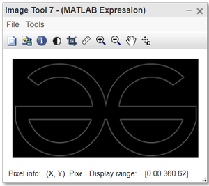
边缘检测图像

中央运营商 [1 0 -1]：

示例 2：

MATLAB

% MATLAB code for Central
% operator edge detection
 k=imread("logo.png");
 k=rgb2gray(k);
 k1=double(k);
 central_msk=[1/2 0 -1/2];
 kx=conv2(k1, central_msk, 'same');
 ky=conv2(k1, central_msk', 'same');
 ked=sqrt(kx.^2 + ky.^2);
   
 %display the images.
 imtool(k,[]);
   
 %display the edge detection along x-axis.
 imtool(kx,[]);
 imtool(abs(kx), []);
   
 %display the edge detection along y-axis.
 imtool(ky,[]);
 imtool(abs(ky),[]); %binarised form
   
 %display the full edge detection.
 imtool(abs(ked),[]);

输出：

在这里，我们可以观察到边缘更加清晰可见。

灰色图像

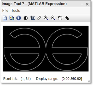
边缘检测图像

向后运算符 [0 1 -1]：

示例 3：

MATLAB

% MATLAB code for Backward
% operator edge detection
k=imread("logo.png");
k=rgb2gray(k);
k1=double(k);
backward_msk=[0 1 -1];
kx=conv2(k1, backward_msk, 'same');
ky=conv2(k1, backward_msk', 'same');
ked=sqrt(kx.^2 + ky.^2);
 
%display the images.
imtool(k,[]);
 
%display the edge detection along x-axis.
imtool(kx,[]);
imtool(abs(kx), []);
 
%display the edge detection along y-axis.
imtool(ky,[]);
imtool(abs(ky),[]);
 
%display the full edge detection.
imtool(ked,[]);
imtool(abs(ked),[]);

输出：

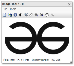
原图

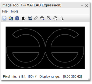
边缘检测图像