机器学习是人工智能的一个子集,专注于开发计算机软件或程序,这些软件或程序可以访问数据以进行自我学习并进行预测,即无需明确编程。机器学习由不同的子部分组成,即无监督学习、监督学习和强化学习。它定义了有助于构建模型的数值问题和分类问题。

R语言用于统计分析和计算,被全世界大多数研究人员使用。 R 正被用于构建机器学习模型,因为它具有灵活性、高效的软件包以及执行与云集成的深度学习模型的能力。作为一种开源语言,所有包都发布在 R 上,并得到了世界各地程序员的贡献,以使其更加用户友好。以下R包在工业中广泛使用的是:
- 数据表
- dplyr
- ggplot2
- 插入符号
- e1071
- xgboost
- 随机森林
数据表
data.table 提供了 R 的 data.frame 的高性能版本,具有功能增强和语法,易于使用、内存高效且功能丰富。它提供了一个快速友好的分隔文件阅读器和文件编写器。它是 Github 上评价最高的软件包之一。它提供低级并行性、具有功能丰富的连接的可扩展聚合以及功能丰富的重塑数据。
R
# Installing the package
install.packages("data.table")

# Loading package
library(data.table)

# Importing dataset
Gov_mortage <- fread("Government_Mortage.csv")

# Record with loan amount 114
# With country code 60
Answer <- Gov_mortage[loan_amount == 114 &
                      county_code == 60]
Answer
R
# Installing the package
install.packages("dplyr")

# Loading package
library(dplyr)

# Importing dataset
Gov_mortage <- fread("Government_Mortage.csv")

# Select
select(Gov_mortage, state_code)

# Mutate
m <- mutate(Gov_mortage,
            amount = loan_amount - applicant_income)
m

# Filter
f = filter(Gov_mortage, county_code == 80)
f

# Arrange
arrange(Gov_mortage, county_code == 80)

# Summarize
summarise(f, max_loan = max(loan_amount))
R
# Installing the package
install.packages("dplyr")
install.packages("ggplot2")

# Loading packages
library(dplyr)
library(ggplot2)

# Data Layer
ggplot(data = mtcars)

# Aesthetic Layer
ggplot(data = mtcars, aes(x = hp,
                          y = mpg,
                          col = disp))

# Geometric layer
ggplot(data = mtcars,
       aes(x = hp, y = mpg,
           col = disp)) + geom_point()
R
# Installing Packages
install.packages("e1071")
install.packages("caTools")
install.packages("caret")

# Loading package
library(e1071)
library(caTools)
library(caret)

# Loading data
data(iris)

# Splitting data into train
# and test data
split <- sample.split(iris, SplitRatio = 0.7)
train_cl <- subset(iris, split == "TRUE")
test_cl <- subset(iris, split == "FALSE")

# Feature Scaling
train_scale <- scale(train_cl[, 1:4])
test_scale <- scale(test_cl[, 1:4])

# Fitting Naive Bayes Model
# to training dataset
set.seed(120)  # Setting Seed
classifier_cl <- naiveBayes(Species ~ .,
                            data = train_cl)
classifier_cl

# Predicting on test data'
y_pred <- predict(classifier_cl,
                  newdata = test_cl)

# Confusion Matrix
cm <- table(test_cl$Species, y_pred)
cm
R
# Installing Packages
install.packages("e1071")
install.packages("caTools")
install.packages("class")

# Loading package
library(e1071)
library(caTools)
library(class)

# Loading data
data(iris)

# Splitting data into train
# and test data
split <- sample.split(iris, SplitRatio = 0.7)
train_cl <- subset(iris, split == "TRUE")
test_cl <- subset(iris, split == "FALSE")

# Feature Scaling
train_scale <- scale(train_cl[, 1:4])
test_scale <- scale(test_cl[, 1:4])

# Fitting KNN Model
# to training dataset
classifier_knn <- knn(train = train_scale,
                      test = test_scale,
                      cl = train_cl$Species,
                      k = 1)
classifier_knn

# Confusiin Matrix
cm <- table(test_cl$Species, classifier_knn)
cm

# Model Evaluation - Choosing K
# Calculate out of Sample error
misClassError <- mean(classifier_knn != test_cl$Species)
print(paste('Accuracy =', 1 - misClassError))
R
# Installing Packages
install.packages("data.table")
install.packages("dplyr")
install.packages("ggplot2")
install.packages("caret")
install.packages("xgboost")
install.packages("e1071")
install.packages("cowplot")

# Loading packages
library(data.table) # for reading and manipulation of data
library(dplyr)      # for data manipulation and joining
library(ggplot2)    # for ploting
library(caret)      # for modeling
library(xgboost)    # for building XGBoost model
library(e1071)      # for skewness
library(cowplot)    # for combining multiple plots

# Setting test dataset
# Combining datasets
# add Item_Outlet_Sales to test data
test[, Item_Outlet_Sales := NA]
combi = rbind(train, test)

# Missing Value Treatment
missing_index = which(is.na(combi$Item_Weight))
for(i in missing_index){
  item = combi$Item_Identifier[i]
  combi$Item_Weight[i] = mean(combi$Item_Weight
                         [combi$Item_Identifier == item],
                         na.rm = T)
}

# Replacing 0 in Item_Visibility with mean
zero_index = which(combi$Item_Visibility == 0)
for(i in zero_index){
  item = combi$Item_Identifier[i]
  combi$Item_Visibility[i] = mean(
       combi$Item_Visibility[combi$Item_Identifier == item],
       na.rm = T)
}

# Label Encoding
# To convert categorical in numerical
combi[, Outlet_Size_num :=
           ifelse(Outlet_Size == "Small", 0,
           ifelse(Outlet_Size == "Medium", 1, 2))]

combi[, Outlet_Location_Type_num :=
           ifelse(Outlet_Location_Type == "Tier 3", 0,
           ifelse(Outlet_Location_Type == "Tier 2", 1, 2))]

combi[, c("Outlet_Size", "Outlet_Location_Type") := NULL]

# One Hot Encoding
# To convert categorical in numerical
ohe_1 = dummyVars("~.",
        data = combi[, -c("Item_Identifier",
                    "Outlet_Establishment_Year",
                    "Item_Type")], fullRank = T)
ohe_df = data.table(predict(ohe_1,
         combi[, -c("Item_Identifier",
         "Outlet_Establishment_Year", "Item_Type")]))

combi = cbind(combi[, "Item_Identifier"], ohe_df)

# Remove skewness
skewness(combi$Item_Visibility)
skewness(combi$price_per_unit_wt)

# log + 1 to avoid division by zero
combi[, Item_Visibility := log(Item_Visibility + 1)]

# Scaling and Centering data
# index of numeric features
num_vars = which(sapply(combi, is.numeric))
num_vars_names = names(num_vars)

combi_numeric = combi[, setdiff(num_vars_names,
                "Item_Outlet_Sales"), with = F]

prep_num = preProcess(combi_numeric,
                 method = c("center", "scale"))
combi_numeric_norm = predict(prep_num, combi_numeric)

# removing numeric independent variables
combi[, setdiff(num_vars_names,
               "Item_Outlet_Sales") := NULL]
combi = cbind(combi,
              combi_numeric_norm)

# Splitting data back to train and test
train = combi[1:nrow(train)]
test = combi[(nrow(train) + 1):nrow(combi)]

# Removing Item_Outlet_Sales
test[, Item_Outlet_Sales := NULL]

# Model Building: XGBoost
param_list = list(
  objective = "reg:linear",
  eta = 0.01,
  gamma = 1,
  max_depth = 6,
  subsample = 0.8,
  colsample_bytree = 0.5
)

# Converting train and test into xgb.DMatrix format
Dtrain = xgb.DMatrix(
         data = as.matrix(train[, -c("Item_Identifier",
                                "Item_Outlet_Sales")]),
         label = train$Item_Outlet_Sales)
Dtest = xgb.DMatrix(
         data = as.matrix(test[, -c("Item_Identifier")]))

# 5-fold cross-validation to
# find optimal value of nrounds
set.seed(112)  # Setting seed
xgbcv = xgb.cv(params = param_list,
               data = Dtrain,
               nrounds = 1000,
               nfold = 5,
               print_every_n = 10,
               early_stopping_rounds = 30,
               maximize = F)

# Training XGBoost model at nrounds = 428
xgb_model = xgb.train(data = Dtrain,
                      params = param_list,
                      nrounds = 428)
xgb_model
R
# Installing package

# For sampling the dataset
install.packages("caTools")

# For implementing random forest algorithm
install.packages("randomForest")

# Loading package
library(caTools)
library(randomForest)

# Loading data
data(iris)

# Splitting data in train and test data
split <- sample.split(iris, SplitRatio = 0.7)
split

train <- subset(iris, split == "TRUE")
test <- subset(iris, split == "FALSE")

# Fitting Random Forest to the train dataset
set.seed(120)  # Setting seed
classifier_RF = randomForest(x = train[-5],
                             y = train$Species,
                             ntree = 500)

classifier_RF

# Predicting the Test set results
y_pred = predict(classifier_RF, newdata = test[-5])

# Confusion Matrix
confusion_mtx = table(test[, 5], y_pred)
confusion_mtx
输出:
row_id loan_type property_type loan_purpose occupancy loan_amount preapproval msa_md
1:     65         1             1            3         1         114           3    344
2:   1285         1             1            1         1         114           2     -1
3:   6748         1             1            3         1         114           3    309
4:  31396         1             1            1         1         114           1    333
5:  70311         1             1            1         1         114           3    309
6: 215535         1             1            3         1         114           3    365
7: 217264         1             1            1         2         114           3    333
8: 301947         1             1            3         1         114           3     48
  state_code county_code applicant_ethnicity applicant_race applicant_sex
1:          9          60                   2              5             1
2:         25          60                   2              5             2
3:         47          60                   2              5             2
4:          6          60                   2              5             1
5:         47          60                   2              5             2
6:         21          60                   2              5             1
7:          6          60                   2              5             1
8:         14          60                   2              5             2
  applicant_income population minority_population_pct ffiecmedian_family_income
1:               68       6355                  14.844                     61840
2:               57       1538                   2.734                     58558
3:               54       4084                   5.329                     76241
4:              116       5445                  41.429                     70519
5:               50       5214                   3.141                     74094
6:               57       6951                   4.219                     56341
7:               37       2416                  18.382                     70031
8:               35       3159                   8.533                     56335
  tract_to_msa_md_income_pct number_of_owner-occupied_units
1:                    100.000                           1493
2:                    100.000                            561
3:                    100.000                           1359
4:                    100.000                           1522
5:                    100.000                           1694
6:                     97.845                           2134
7:                     65.868                            905
8:                    100.000                           1080
  number_of_1_to_4_family_units lender co_applicant
1:                          2202   3507         TRUE
2:                           694   6325        FALSE
3:                          1561   3549        FALSE
4:                          1730   2111         TRUE
5:                          2153   3229        FALSE
6:                          2993   1574         TRUE
7:                          3308   3110        FALSE
8:                          1492   6314        FALSE
Dplyr
Dplyr 是业界广泛使用的数据操作包。它由五个关键的数据操作函数组成,也称为动词,即选择、过滤、排列、变异和汇总。
电阻
# Installing the package
install.packages("dplyr")

# Loading package
library(dplyr)

# Importing dataset
Gov_mortage <- fread("Government_Mortage.csv")

# Select
select(Gov_mortage, state_code)

# Mutate
m <- mutate(Gov_mortage,
            amount = loan_amount - applicant_income)
m

# Filter
f = filter(Gov_mortage, county_code == 80)
f

# Arrange
arrange(Gov_mortage, county_code == 80)

# Summarize
summarise(f, max_loan = max(loan_amount))
输出:
# Filter
row_id loan_type property_type loan_purpose occupancy loan_amount preapproval msa_md
1 16 1 1 3 2 177 3 333
2 25 1 1 3 1 292 3 333
3 585 1 1 3 1 134 3 333
4 1033 1 1 1 1 349 2 333
5 1120 1 1 1 1 109 3 333
6 1303 1 1 3 2 166 3 333
7 1758 1 1 2 1 45 3 333
8 2053 3 1 1 1 267 3 333
9 3305 1 1 3 1 392 3 333
10 3555 1 1 3 1 98 3 333
11 3769 1 1 3 1 288 3 333
12 3807 1 1 1 1 185 3 333
13 3840 1 1 3 1 280 3 333
14 5356 1 1 3 1 123 3 333
15 5604 2 1 1 1 191 1 333
16 6294 1 1 2 1 102 3 333
17 7631 3 1 3 1 107 3 333
18 8222 2 1 3 1 62 3 333
19 9335 1 1 3 1 113 3 333
20 10137 1 1 1 1 204 3 333
21 10387 3 1 1 1 434 2 333
22 10601 2 1 1 1 299 2 333
23 13076 1 1 1 1 586 3 333
24 13763 1 1 3 1 29 3 333
25 13769 3 1 1 1 262 3 333
26 13818 2 1 1 1 233 3 333
27 14102 1 1 3 1 130 3 333
28 14196 1 1 2 1 3 3 333
29 15569 1 1 1 1 536 2 333
30 15863 1 1 1 1 20 3 333
31 16184 1 1 3 1 755 3 333
32 16296 1 1 1 2 123 2 333
33 16328 1 1 3 1 153 3 333
34 16486 3 1 3 1 95 3 333
35 16684 1 1 2 1 26 3 333
36 16922 1 1 1 1 160 2 333
37 17470 1 1 3 1 174 3 333
38 18336 1 2 1 1 37 3 333
39 18586 1 2 1 1 114 3 333
40 19249 1 1 3 1 422 3 333
41 19405 1 1 1 1 288 2 333
42 19421 1 1 2 1 301 3 333
43 20125 1 1 3 1 449 3 333
44 20388 1 1 1 1 494 3 333
45 21434 1 1 3 1 251 3 333
state_code county_code applicant_ethnicity applicant_race applicant_sex
1 6 80 1 5 2
2 6 80 2 3 2
3 6 80 2 5 2
4 6 80 3 6 1
5 6 80 2 5 2
6 6 80 1 5 1
7 6 80 2 5 1
8 6 80 1 5 2
9 6 80 2 5 1
10 6 80 2 5 1
11 6 80 2 5 1
12 6 80 1 5 1
13 6 80 1 5 1
14 6 80 1 5 1
15 6 80 2 5 1
16 6 80 2 5 1
17 6 80 3 6 3
18 6 80 2 5 1
19 6 80 2 5 2
20 6 80 2 5 1
21 6 80 2 5 1
22 6 80 2 5 1
23 6 80 3 6 3
24 6 80 2 5 2
25 6 80 2 5 1
26 6 80 2 5 1
27 6 80 2 5 2
28 6 80 1 6 1
29 6 80 2 5 1
30 6 80 2 5 1
31 6 80 2 5 1
32 6 80 2 5 2
33 6 80 1 5 1
34 6 80 2 5 1
35 6 80 2 5 1
36 6 80 2 5 2
37 6 80 2 5 1
38 6 80 1 5 1
39 6 80 1 5 1
40 6 80 1 5 1
41 6 80 2 2 1
42 6 80 2 5 1
43 6 80 2 5 1
44 6 80 2 5 1
45 6 80 2 5 1
applicant_income population minority_population_pct ffiecmedian_family_income
1 NA 6420 29.818 68065
2 99 4346 16.489 70745
3 46 6782 20.265 69818
4 236 9813 15.168 69691
5 49 5854 35.968 70555
6 148 4234 19.864 72156
7 231 5699 17.130 71892
8 48 6537 13.024 71562
9 219 18911 26.595 69795
10 71 8454 17.436 68727
11 94 6304 13.490 69181
12 78 9451 14.684 69337
13 74 15540 43.148 70000
14 54 16183 42.388 70862
15 73 11198 40.481 70039
16 199 12133 10.971 70023
17 43 10712 33.973 68117
18 115 8759 17.669 70526
19 59 24887 32.833 71510
20 135 25252 31.854 69602
21 108 6507 13.613 70267
22 191 9261 22.583 71505
23 430 7943 19.990 70801
24 206 7193 18.002 69973
25 150 7413 14.092 68202
26 94 7611 14.618 71260
27 81 10946 34.220 70386
28 64 10438 36.395 70141
29 387 8258 20.666 69409
30 80 7525 26.604 70104
31 NA 4525 20.299 71947
32 40 8397 32.542 68087
33 87 20083 19.750 69893
34 96 20539 19.673 72152
35 45 10497 12.920 70134
36 54 15686 26.071 70890
37 119 7558 14.710 69052
38 62 25960 32.858 68061
39 18 5790 39.450 68878
40 103 18086 26.099 69925
41 70 8689 31.467 70794
42 38 3923 30.206 68821
43 183 6522 13.795 69779
44 169 18459 26.874 69392
45 140 15954 25.330 71096
tract_to_msa_md_income_pct number_of_owner-occupied_units
1 100.000 1553
2 100.000 1198
3 100.000 1910
4 100.000 2351
5 100.000 1463
6 100.000 1276
7 100.000 1467
8 100.000 1766
9 100.000 4316
10 90.071 2324
11 100.000 1784
12 100.000 2357
13 100.000 3252
14 100.000 3319
15 79.049 2438
16 100.000 3639
17 100.000 2612
18 87.201 2345
19 100.000 6713
20 100.000 6987
21 100.000 1788
22 91.023 2349
23 100.000 1997
24 100.000 2012
25 100.000 2359
26 100.000 2304
27 100.000 2674
28 80.957 2023
29 100.000 2034
30 100.000 2343
31 77.707 1059
32 100.000 1546
33 100.000 5929
34 100.000 6017
35 100.000 3542
36 100.000 4277
37 100.000 2316
38 100.000 6989
39 56.933 1021
40 100.000 4183
41 100.000 1540
42 100.000 882
43 100.000 1774
44 100.000 4417
45 100.000 4169
number_of_1_to_4_family_units lender co_applicant
1 2001 3354 FALSE
2 1349 2458 FALSE
3 2326 4129 FALSE
4 2928 4701 TRUE
5 1914 2134 FALSE
6 1638 5710 FALSE
7 1670 3110 FALSE
8 1926 3080 TRUE
9 5241 5710 TRUE
10 3121 5710 FALSE
11 1953 933 FALSE
12 2989 186 TRUE
13 4482 2134 TRUE
14 4380 5339 TRUE
15 3495 5267 TRUE
16 4875 1831 TRUE
17 3220 5710 FALSE
18 3024 3885 TRUE
19 7980 2458 FALSE
20 7949 6240 TRUE
21 2015 542 TRUE
22 3215 2702 TRUE
23 2361 3216 FALSE
24 2482 6240 FALSE
25 2597 3970 TRUE
26 2503 3264 FALSE
27 3226 2570 TRUE
28 3044 6240 FALSE
29 2423 1928 TRUE
30 2659 5738 FALSE
31 1544 2458 FALSE
32 2316 3950 FALSE
33 7105 3143 FALSE
34 7191 4701 FALSE
35 4325 5339 FALSE
36 5188 2702 FALSE
37 2531 2458 TRUE
38 7976 2318 TRUE
39 1755 5026 FALSE
40 5159 4931 TRUE
41 2337 2352 FALSE
42 1317 2458 FALSE
43 1949 5726 FALSE
44 5055 5316 TRUE
45 5197 5726 FALSE
[ reached 'max' / getOption("max.print") -- omitted 1034 rows ]
#
ggplot2
ggplot2 也称为Grammer of Graphics是一个免费、开源且易于使用的可视化包,广泛应用于 R 中。它是 Hadley Wickham 编写的最强大的可视化包。
电阻
# Installing the package
install.packages("dplyr")
install.packages("ggplot2")

# Loading packages
library(dplyr)
library(ggplot2)

# Data Layer
ggplot(data = mtcars)

# Aesthetic Layer
ggplot(data = mtcars, aes(x = hp,
                          y = mpg,
                          col = disp))

# Geometric layer
ggplot(data = mtcars,
       aes(x = hp, y = mpg,
           col = disp)) + geom_point()
输出:
- 几何层:

- 几何层 – 添加大小:

插入符号
称为分类和回归训练的插入符号使用许多函数来训练和绘制分类和回归模型。它是 R 开发人员和各种机器学习竞赛中使用最广泛的软件包之一。
电阻
# Installing Packages
install.packages("e1071")
install.packages("caTools")
install.packages("caret")

# Loading package
library(e1071)
library(caTools)
library(caret)

# Loading data
data(iris)

# Splitting data into train
# and test data
split <- sample.split(iris, SplitRatio = 0.7)
train_cl <- subset(iris, split == "TRUE")
test_cl <- subset(iris, split == "FALSE")

# Feature Scaling
train_scale <- scale(train_cl[, 1:4])
test_scale <- scale(test_cl[, 1:4])

# Fitting Naive Bayes Model
# to training dataset
set.seed(120)  # Setting Seed
classifier_cl <- naiveBayes(Species ~ .,
                            data = train_cl)
classifier_cl

# Predicting on test data'
y_pred <- predict(classifier_cl,
                  newdata = test_cl)

# Confusion Matrix
cm <- table(test_cl$Species, y_pred)
cm
输出:
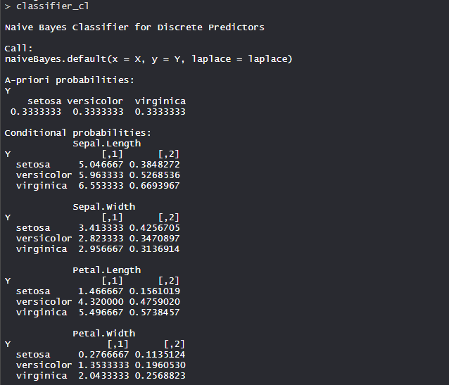
- 模型分类器_cl:
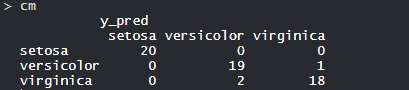
- 混淆矩阵:
e1071
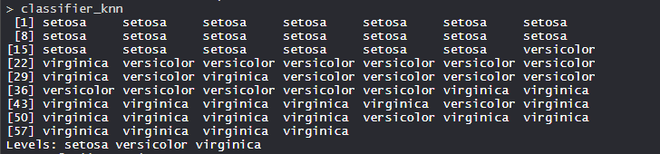
e1071包用于执行聚类算法、支持向量机(SVM)、最短路径计算、袋装聚类算法、K-NN 算法等。主要用于执行 K-NN 算法。这取决于它的 k 值(邻居),并在金融行业、医疗保健行业等许多行业找到它的应用。 K-最近邻居或 K-NN 是一种监督非线性分类算法。 K-NN 是一种非参数算法,即它不对基础数据或其分布做出任何假设。
电阻
# Installing Packages
install.packages("e1071")
install.packages("caTools")
install.packages("class")

# Loading package
library(e1071)
library(caTools)
library(class)

# Loading data
data(iris)

# Splitting data into train
# and test data
split <- sample.split(iris, SplitRatio = 0.7)
train_cl <- subset(iris, split == "TRUE")
test_cl <- subset(iris, split == "FALSE")

# Feature Scaling
train_scale <- scale(train_cl[, 1:4])
test_scale <- scale(test_cl[, 1:4])

# Fitting KNN Model
# to training dataset
classifier_knn <- knn(train = train_scale,
                      test = test_scale,
                      cl = train_cl$Species,
                      k = 1)
classifier_knn

# Confusiin Matrix
cm <- table(test_cl$Species, classifier_knn)
cm

# Model Evaluation - Choosing K
# Calculate out of Sample error
misClassError <- mean(classifier_knn != test_cl$Species)
print(paste('Accuracy =', 1 - misClassError))
输出:
- 模型分类器_knn(k=1):
- 混淆矩阵:

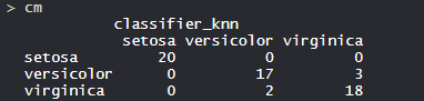
- 模型评估(k=1):

XGBoost
XGBoost仅适用于数字变量。它是提升技术的一部分,其中更智能地选择样本以对观察进行分类。在 C++、R、 Python、Julia、 Java和 Scala 中有 XGBoost 的接口。它由Bagging和Boosting技术组成。数据集使用BigMart 。
电阻
# Installing Packages
install.packages("data.table")
install.packages("dplyr")
install.packages("ggplot2")
install.packages("caret")
install.packages("xgboost")
install.packages("e1071")
install.packages("cowplot")
# Loading packages
library(data.table) # for reading and manipulation of data
library(dplyr) # for data manipulation and joining
library(ggplot2) # for ploting
library(caret) # for modeling
library(xgboost) # for building XGBoost model
library(e1071) # for skewness
library(cowplot) # for combining multiple plots
# Setting test dataset
# Combining datasets
# add Item_Outlet_Sales to test data
test[, Item_Outlet_Sales := NA]
combi = rbind(train, test)
# Missing Value Treatment
missing_index = which(is.na(combi$Item_Weight))
for(i in missing_index){
item = combi$Item_Identifier[i]
combi$Item_Weight[i] = mean(combi$Item_Weight
[combi$Item_Identifier == item],
na.rm = T)
}
# Replacing 0 in Item_Visibility with mean
zero_index = which(combi$Item_Visibility == 0)
for(i in zero_index){
item = combi$Item_Identifier[i]
combi$Item_Visibility[i] = mean(
combi$Item_Visibility[combi$Item_Identifier == item],
na.rm = T)
}
# Label Encoding
# To convert categorical in numerical
combi[, Outlet_Size_num :=
ifelse(Outlet_Size == "Small", 0,
ifelse(Outlet_Size == "Medium", 1, 2))]
combi[, Outlet_Location_Type_num :=
ifelse(Outlet_Location_Type == "Tier 3", 0,
ifelse(Outlet_Location_Type == "Tier 2", 1, 2))]
combi[, c("Outlet_Size", "Outlet_Location_Type") := NULL]
# One Hot Encoding
# To convert categorical in numerical
ohe_1 = dummyVars("~.",
data = combi[, -c("Item_Identifier",
"Outlet_Establishment_Year",
"Item_Type")], fullRank = T)
ohe_df = data.table(predict(ohe_1,
combi[, -c("Item_Identifier",
"Outlet_Establishment_Year", "Item_Type")]))
combi = cbind(combi[, "Item_Identifier"], ohe_df)
# Remove skewness
skewness(combi$Item_Visibility)
skewness(combi$price_per_unit_wt)
# log + 1 to avoid division by zero
combi[, Item_Visibility := log(Item_Visibility + 1)]
# Scaling and Centering data
# index of numeric features
num_vars = which(sapply(combi, is.numeric))
num_vars_names = names(num_vars)
combi_numeric = combi[, setdiff(num_vars_names,
"Item_Outlet_Sales"), with = F]
prep_num = preProcess(combi_numeric,
method = c("center", "scale"))
combi_numeric_norm = predict(prep_num, combi_numeric)
# removing numeric independent variables
combi[, setdiff(num_vars_names,
"Item_Outlet_Sales") := NULL]
combi = cbind(combi,
combi_numeric_norm)
# Splitting data back to train and test
train = combi[1:nrow(train)]
test = combi[(nrow(train) + 1):nrow(combi)]
# Removing Item_Outlet_Sales
test[, Item_Outlet_Sales := NULL]
# Model Building: XGBoost
param_list = list(
objective = "reg:linear",
eta = 0.01,
gamma = 1,
max_depth = 6,
subsample = 0.8,
colsample_bytree = 0.5
)
# Converting train and test into xgb.DMatrix format
Dtrain = xgb.DMatrix(
data = as.matrix(train[, -c("Item_Identifier",
"Item_Outlet_Sales")]),
label = train$Item_Outlet_Sales)
Dtest = xgb.DMatrix(
data = as.matrix(test[, -c("Item_Identifier")]))
# 5-fold cross-validation to
# find optimal value of nrounds
set.seed(112) # Setting seed
xgbcv = xgb.cv(params = param_list,
data = Dtrain,
nrounds = 1000,
nfold = 5,
print_every_n = 10,
early_stopping_rounds = 30,
maximize = F)
# Training XGBoost model at nrounds = 428
xgb_model = xgb.train(data = Dtrain,
params = param_list,
nrounds = 428)
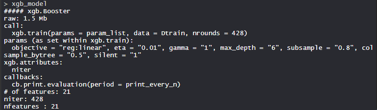
xgb_model
输出:
- Xgboost模型的训练:
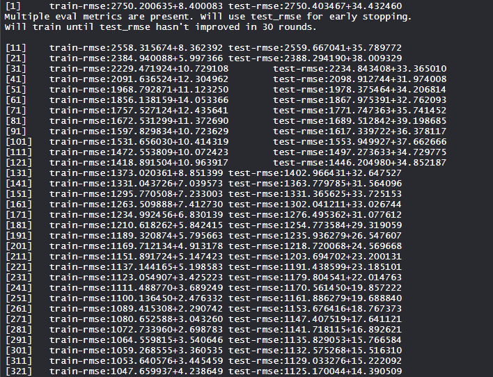
- 型号 xgb_model:
随机森林
R 编程中的随机森林是决策树的集合。它构建并组合多个决策树以获得更准确的预测。这是一种非线性分类算法。每个决策树模型在单独使用时都会使用。构建树时不使用案例的错误估计。这称为以百分比形式提及的袋外误差估计。
电阻
# Installing package

# For sampling the dataset
install.packages("caTools")

# For implementing random forest algorithm
install.packages("randomForest")

# Loading package
library(caTools)
library(randomForest)

# Loading data
data(iris)

# Splitting data in train and test data
split <- sample.split(iris, SplitRatio = 0.7)
split

train <- subset(iris, split == "TRUE")
test <- subset(iris, split == "FALSE")

# Fitting Random Forest to the train dataset
set.seed(120)  # Setting seed
classifier_RF = randomForest(x = train[-5],
                             y = train$Species,
                             ntree = 500)

classifier_RF

# Predicting the Test set results
y_pred = predict(classifier_RF, newdata = test[-5])

# Confusion Matrix
confusion_mtx = table(test[, 5], y_pred)
confusion_mtx
输出:
- 模型分类器_RF:
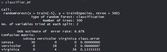
- 混淆矩阵: