Excel 包含许多有用的函数,这样的函数就是“MATCH()”函数。它基本上用于从一系列单元格(即从行或列或从表格)中获取特定项目的相对位置。此函数还支持像VLOOKUP()函数一样的精确和近似匹配。通常,MATCH()函数与 INDEX()函数。
在 MATCH()函数的帮助下,用户可以从表格或单元格范围中获取特定元素的相对位置。相对位置是指元素在 MATCH()函数搜索元素所在的行或列中的位置。准确地说,这个函数帮助我们获取数组中元素的位置。
句法:
=MATCH(lookup_value, lookup_array, [match_type])这里,[match_type] 值表示用户想要精确匹配还是近似匹配。
参数:
- lookup_value(必需):它是用户想要搜索的值(文本或数字或逻辑值或包含数字、文本或逻辑值的单元格引用)。此参数必须由用户提供。
- lookup_array(必需):此参数包含单元格范围或对数组的引用,MATCH()函数将在其中尝试找出 lookup_value。同样,此参数必须由用户提供。
- [match_type](可选):这是一个可选参数。该值可能是 1、0 或 -1。如果值为 0,则用户需要精确匹配。如果值为 1 MATCH()函数将返回小于或等于lookup_value 的最大值,如果值为 -1 则函数将返回大于或等于lookup_value的最小值。
Note: If [match_type] argument is 1 or -1 then the lookup_array must be in a sorted order(ascending for 1 and descending for -1) and if the argument is not provided by the user the value becomes 1 by default.
返回值:此函数返回一个值,该值表示查找值在一系列单元格中的相对位置。
例子:
下面给出了 MATCH()函数的示例。列表中使用的名称仅用于示例目的,与任何真实人物无关。
| Student Names | Age | Phone Numbers | Roll No. |
|---|---|---|---|
| Amod Yadav | 21 | 9123456789 | 1010 |
| Sukanya Tripathi | 20 | 2345685523 | 1011 |
| Vijay Chaurasia | 19 | 1256485421 | 1012 |
| Abhisekh Upmanyu | 18 | 6665551110 | 1013 |
| Dinesh Shukla | 17 | 6026452364 | 1014 |
| Vineeta Tiwari | 16 | 2154832564 | 1015 |
| Vineeta Tiwari | 15 | 5214563254 | 1016 |
| Chand Podder | 14 | 3215648866 | 1017 |
例如使用上面的列表。
| Formula | Result | Remarks |
|---|---|---|
| MATCH(A9, A1:A9, 0) | 9 | MATCH function searches for an exact match and returns the relative position of the element. |
| MATCH(1018, D1:D9) | 9 |
Here [match_type] argument is omitted so the value is 1 and the function searches for an approximate match and returns the position of the next greater element in the list. |
| MATCH(“CHAND PODDER”, A1:A9, 0) | 9 | This output proves that the MATCH function is not case-sensitive. |
| MATCH(“Vineeta Tiwari”, A1:A9, 0) | 7 | MATCH function always returns the position of the first match. |
| MATCH(13, B1:B9, -1) | 9 |
Here [match_type] argument is -1 and the function searches for an approximate match and returns the position of the next smallest element in the list. |
下面是 Excel 工作表的输出屏幕截图。
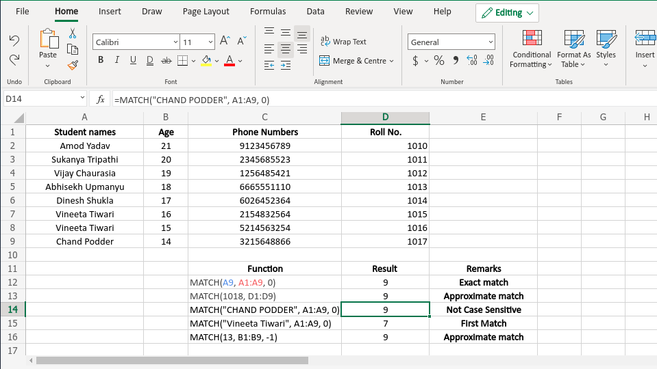
输出截图