Python的蒙特卡罗集成

蒙特卡洛积分是求解具有大量积分值的积分的过程。蒙特卡罗过程使用大数理论和随机抽样来逼近非常接近积分实际解的值。它对表示的函数的平均值函数。然后我们可以将 扩展为值的总和除以积分中的点数，并求解方程的左侧以近似右侧的积分值。推导如下。

$<f(x)> = \frac{1}{b-a} \int_{a}^{b} f(x) \,dx \newline (b-a) <f(x)> = \int_{a}^{b} f(x) \,dx \newline (b-a) \frac{1}{N} \sum_{i=1}^{N} f(x_i) \approx \int_{a}^{b} f(x) \,dx$

其中 N = 否。用于近似值的术语。

现在我们将首先使用蒙特卡罗方法以数值方式计算积分，然后最后我们将使用Python库 matplotlib 使用直方图可视化结果。

使用的模块：

将使用的模块是：

• Scipy ：用于获取积分极限之间的随机值。可以使用以下方式安装：

pip install scipy # for windows
or
pip3 install scipy # for linux and macos

• Numpy ：用于形成数组并存储不同的值。可以使用以下方式安装：

pip install numpy # for windows
or 
pip3 install numpy # for linux and macos

• Matplotlib ：用于可视化直方图和蒙特卡罗积分的结果。

pip install matplotlib # for windows
or 
pip3 install matplotlib # for linux and macos

示例 1：

我们要评估的积分是：

一旦我们完成安装模块，我们现在可以通过导入所需的模块开始编写代码，用于在范围内创建随机值的 scipy 和用于创建静态数组的 NumPy 模块，因为在Python中由于动态内存分配相对较慢。然后我们定义了积分的限制，即 0 和 pi（我们使用 np.pi 来获取 pi 的值。然后我们使用 np.zeros(N) 创建一个大小为 N 的零的静态 numpy 数组。现在我们迭代数组 N 的每个索引并用 a 和 b 之间的随机值填充它。然后我们创建一个变量来存储整数变量不同值的函数之和。现在我们创建一个函数来计算 x 的特定值的 sin . 然后我们对x的不同值的x的函数返回的所有值进行迭代，将所有的值相加到变量积分中，然后我们使用上面推导出来的公式得到结果，最后我们将结果打印在最后一行。

Python3

# importing the modules
from scipy import random
import numpy as np
 
# limits of integration
a = 0
b = np.pi # gets the value of pi
N = 1000
 
# array of zeros of length N
ar = np.zeros(N)
 
# iterating over each Value of ar and filling
# it with a random value between the limits a
# and b
for i in range (len(ar)):
    ar[i] = random.uniform(a,b)
 
# variable to store sum of the functions of
# different values of x
integral = 0.0
 
# function to calculate the sin of a particular
# value of x
def f(x):
    return np.sin(x)
 
# iterates and sums up values of different functions
# of x
for i in ar:
    integral += f(i)
 
# we get the answer by the formula derived adobe
ans = (b-a)/float(N)*integral
 
# prints the solution
print ("The value calculated by monte carlo integration is {}.".format(ans))

输出：

The value calculated by monte carlo integration is 2.0256756150767035.

获得的值非常接近积分的实际答案 2.0。

现在，如果我们想使用直方图可视化集成，我们可以使用 matplotlib 库来实现。我们再次导入模块，定义积分极限并编写 sin函数来计算特定 x 值的 sin 值。接下来，我们采用一个数组，该数组的变量代表直方图的每个光束。然后我们迭代 N 个值并重复创建零数组的相同过程，用随机 x 值填充它，创建一个积分变量，将所有函数值相加，并得到 N 次答案，每个答案代表直方图的一个光束.代码如下：

蟒蛇3

# importing the modules
from scipy import random
import numpy as np
import matplotlib.pyplot as plt
 
# limits of integration
a = 0
b = np.pi # gets the value of pi
N = 1000
 
# function to calculate the sin of a particular
# value of x
def f(x):
    return np.sin(x)
 
# list to store all the values for plotting
plt_vals = []
 
# we iterate through all the values to generate
# multiple results and show whose intensity is
# the most.
for i in range(N):
   
    #array of zeros of length N
    ar = np.zeros(N)
 
    # iterating over each Value of ar and filling it
    # with a randome value between the limits a and b
    for i in range (len(ar)):
        ar[i] = random.uniform(a,b)
 
    # variable to store sum of the functions of different
    # values of x
    integral = 0.0
 
    # iterates and sums up values of different functions
    # of x
    for i in ar:
        integral += f(i)
 
    # we get the answer by the formula derived adobe
    ans = (b-a)/float(N)*integral
 
    # appends the solution to a list for plotting the graph
    plt_vals.append(ans)
 
# details of the plot to be generated
# sets the title of the plot
plt.title("Distributions of areas calculated")
 
# 3 parameters (array on which histogram needs
plt.hist (plt_vals, bins=30, ec="black")
 
# to be made, bins, separators colour between the
# beams)
# sets the label of the x-axis of the plot
plt.xlabel("Areas")
plt.show() # shows the plot

输出：

正如我们所看到的，根据该图，最可能的结果是 2.023 或 2.024，这再次非常接近该积分的实际解 2.0。

示例 2：

我们要评估的积分是：

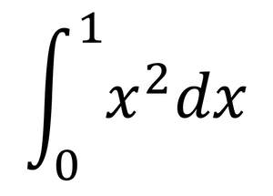
实现将与上一个问题相同，只有 a 和 b 定义的积分限制会改变，并且返回特定值的相应函数值的 f(x)函数现在将返回 x^2 而不是 sin （X）。这个代码是：

蟒蛇3

# importing the modules
from scipy import random
import numpy as np
 
# limits of integration
a = 0
b = 1
N = 1000
 
# array of zeros of length N
ar = np.zeros(N)
 
# iterating over each Value of ar and filling
# it with a random value between the limits a
# and b
for i in range(len(ar)):
    ar[i] = random.uniform(a, b)
 
# variable to store sum of the functions of
# different values of x
integral = 0.0
 
# function to calculate the sin of a particular
# value of x
def f(x):
    return x**2
 
# iterates and sums up values of different
# functions of x
for i in ar:
    integral += f(i)
 
# we get the answer by the formula derived adobe
ans = (b-a)/float(N)*integral
 
# prints the solution
print("The value calculated by monte carlo integration is {}.".format(ans))

输出：

The value calculated by monte carlo integration is 0.33024026610116575.

获得的值非常接近积分的实际答案 0.333。

现在，如果我们想再次使用直方图可视化积分，我们可以使用 matplotlib 库来实现，就像我们在前面的期望中所做的那样，在这种情况下，f(x) 函数返回 x^2 而不是 sin(x)，并且积分极限由0变为1，代码如下：

蟒蛇3

# importing the modules
from scipy import random
import numpy as np
import matplotlib.pyplot as plt
 
# limits of integration
a = 0
b = 1
N = 1000
 
# function to calculate x^2 of a particular value
# of x
def f(x):
    return x**2
 
# list to store all the values for plotting
plt_vals = []
 
# we iterate through all the values to generate
# multiple results and show whose intensity is
# the most.
for i in range(N):
   
    # array of zeros of length N
    ar = np.zeros(N)
 
    # iterating over each Value of ar and filling
    # it with a randome value between the limits a
    # and b
    for i in range (len(ar)):
        ar[i] = random.uniform(a,b)
 
    # variable to store sum of the functions of
    # different values of x
    integral = 0.0
 
    # iterates and sums up values of different functions
    # of x
    for i in ar:
        integral += f(i)
 
    # we get the answer by the formula derived adobe
    ans = (b-a)/float(N)*integral
 
    # appends the solution to a list for plotting the
    # graph
    plt_vals.append(ans)
 
# details of the plot to be generated
# sets the title of the plot
plt.title("Distributions of areas calculated")
 
# 3 parameters (array on which histogram needs
# to be made, bins, separators colour between
# the beams)
plt.hist (plt_vals, bins=30, ec="black")
 
# sets the label of the x-axis of the plot
plt.xlabel("Areas")
plt.show() # shows the plot

输出：

正如我们所看到的，根据该图最可能的结果是 0.33，这几乎等于（在这种情况下等于，但通常不会发生）该积分的实际解 0.333。