Julia 中的逻辑回归

顾名思义，逻辑回归在功能上完全相反。逻辑回归基本上是机器学习中用于二元分类的预测算法。它预测类的概率，然后根据预测变量的值对其进行分类。

逻辑回归中的因变量(y)是二进制的，有 2 个可能的值 0 或 1。例如：如果我们要检查邮件是否是垃圾邮件。然后 y 将具有值 - 1 表示垃圾邮件，0 表示非垃圾邮件。

逻辑回归在某些方面类似于线性回归，只是在线性回归中y是一个连续变量，而在逻辑回归中y需要介于0和1之间。因为，y只是预测值，预测值只是y 的概率等于 1, P(y = 1) 。

我们知道，线性回归方程：

$y = b_{0} + b_{1}\times x$

现在，我们知道这个方程产生了一个连续的 y 值。为了将 y 的预测值限制在 0 – 1 范围内，我们应用了 sigmoid函数。 sigmoid函数是，

$P = \frac{1}{1+ e^{-y}}$

由上式计算 y 的值，然后代入线性回归方程，我们得到：

$ln(\frac{P}{1-P}) = b_{0} + b_{1}\times x$

因此，我们最终得到了逻辑回归的方程。使用这个方程，我们可以找到当 x 的值已知时 y 的概率值。在上述等式中，b ₀是截距，b ₁是所有 x 值的斜率矩阵。统称为回归系数。

要了解更多信息，我将以流失建模数据为例，这是一个众所周知的数据集，可根据许多特征预测客户是否流失。让我们从 Julia 开始。

步骤 1：导入包

在这一步中，我们将导入我们将使用的所有必需的包。如果您错过任何包，请不要害怕，您绝对可以同时添加它。

Julia

# Import the packages
import Pkg; 
Pkg.add("Lathe")
using Lathe
  
import Pkg;
Pkg.add("DataFrames")
using DataFrames
  
import Pkg; 
Pkg.add("Plots")
using Plots;
  
import Pkg; 
Pkg.add("GLM")
using GLM
  
import Pkg; 
Pkg.add("StatsBase")
using StatsBase
  
import Pkg; 
Pkg.add("MLBase")
using MLBase
  
import Pkg; 
Pkg.add("ROCAnalysis")
using ROCAnalysis
  
import Pkg; 
Pkg.add("CSV")
using CSV
  
println("Successfully imported the packages!!")

输出：

Successfully imported the packages!!

第 2 步：加载数据集

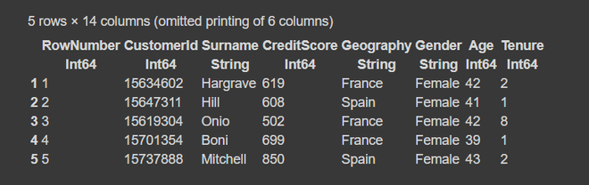
要读取数据，我们使用CSV.file函数，然后使用DataFrame函数将其转换为数据框。

朱莉娅

# Load the data
df = DataFrame(CSV.File("churn modelling.csv"))
first(df, 5)

输出：

第 3 步：数据框摘要

朱莉娅

# Summary of dataframe
println(size(df))
describe(df)

输出：

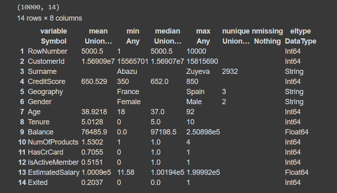
在这种情况下，因变量 y 是最后一列('Exited') 。第一列只是行号，第二列的变量是预测变量或自变量。此外，我们的数据集大小为10,000 行和 14 列。从摘要中，我们发现数据集没有缺失值或空值。列名中没有任何空格或特殊字符，因此我们可以毫无问题地更进一步。

朱莉娅

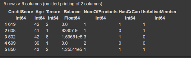
select!(df, Not([:RowNumber, :CustomerId, :Surname, :Geography, :Gender]))
first(df, 5)

输出：

第 4 步：将数据拆分为训练集和测试集。

朱莉娅

# Train test split
using Lathe.preprocess: TrainTestSplit
train, test = TrainTestSplit(df, .75);

第 5 步：建立我们的 Logistic 回归模型。

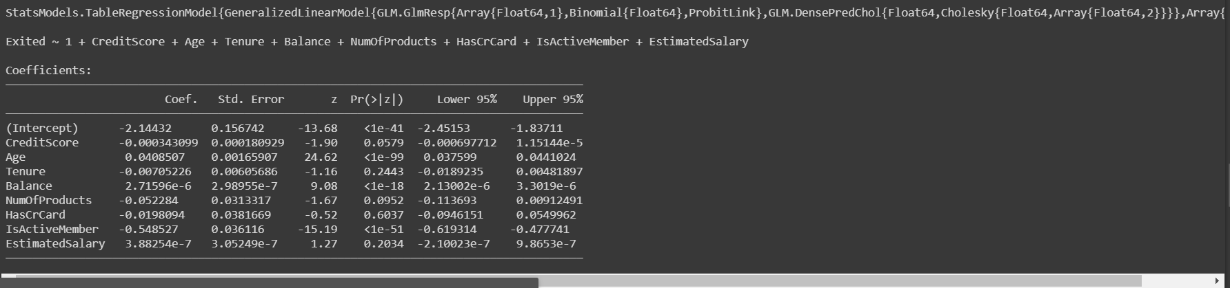
我们使用glm函数进行逻辑回归。

朱莉娅

# Train logistic regression model
fm = @formula(Exited ~ CreditScore + Age + Tenure + 
              Balance + NumOfProducts + HasCrCard + 
              IsActiveMember + EstimatedSalary)
logit = glm(fm, train, Binomial(), ProbitLink())

输出：

一旦我们建立了我们的模型并对其进行了训练，我们将在测试数据上评估模型以查看其工作的准确性。

第 6 步：模型预测和评估

朱莉娅

# Predict the target variable on test data 
prediction = predict(logit, test)

输出：

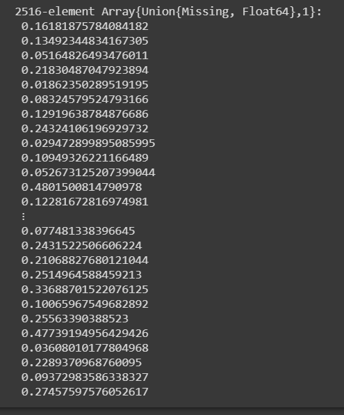
glm 模型为我们提供了第 1 类的概率分数。在获得概率分数后，我们需要根据阈值分数将其分类为 0 或 1。通常，阈值被认为是 0.5。

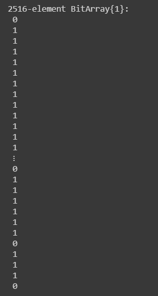
借助上面的代码，我们得到了概率分数。现在，让我们将它们转换为 0 或 1 类。对于概率 > 0.5 将被赋予 1 类，否则为 0。

朱莉娅

# Converting probability score to classes
prediction_class = [if x < 0.5 0 else 1 end for x in prediction];
  
prediction_df = DataFrame(y_actual = test.Exited,
                          y_predicted = prediction_class, 
                          prob_predicted = prediction);
prediction_df.correctly_classified = prediction_df.y_actual .== prediction_df.y_predicted

输出：

在预测我们测试数据的类别之后，下一步是通过分析准确性来评估模型。

步骤 7：计算模型的准确度

准确率是指我们的模型正确预测的类别总数。

朱莉娅

# Finding the Accuracy Score
accuracy = mean(prediction_df.correctly_classified)

输出：

0.7996820349761526

因此，我们的模型产生了大约 80% 的准确率，这是一个很好的分数。现在，为了更好地了解准确性，我们分析了混淆矩阵。

第 8 步：混淆矩阵

混淆矩阵只是评估任何分类模型性能的另一种方式。

朱莉娅

# confusion matrix 
confusion_matrix = MLBase.roc(prediction_df.y_actual, 
                              prediction_df.y_predicted)

输出：

ROCNums{Int64}
  p = 523
  n = 1993
  tp = 69
  tn = 1943
  fp = 50
  fn = 454

上面的输出告诉我们，由于类别不平衡，我们的模型将最大观察值分类为 0 类。这就是 80% 中等准确率的原因。