R编程中的指数平滑

指数平滑是一种使用指数窗口函数平滑时间序列数据的技术。这是经验法则。与简单的移动平均线不同，随着时间的推移，指数函数分配的权重呈指数下降。在这里，较大的权重放在最近的值或观察值上，而较小的权重放在较旧的值或观察值上。在众多窗函数中，在信号处理中，指数平滑函数通常用于平滑数据，它充当低通滤波器以去除高频噪声。这种方法非常直观，一般可以应用于大范围或大范围的时间序列，计算效率也很高。在本文中，让我们讨论 R 编程中的指数平滑。基于趋势和季节性的指数平滑技术有很多种，如下所示：

• 简单指数平滑
• 霍尔特方法
• Holt-Winter 的季节性方法
• 阻尼趋势法

在继续之前，需要查看复制要求。

R中分析的复制要求

在 R 中，此分析的先决条件是安装所需的包。我们需要使用 R 控制台中的install.packages()命令安装以下两个包：

• fpp2 （将自动加载预测包）
• tidyverse

在预测包下，我们将获得许多可以增强和帮助我们预测的功能。在此分析中，我们将使用fpp2包下的两个数据集。这些是“goog”数据集和“qcement”数据集。现在我们需要使用library()函数在我们的 R 脚本中加载所需的包。加载两个包后，我们将准备我们的数据集。对于这两个数据集，我们将数据分为两组，训练集和测试集。

R

# loading the required packages
library(tidyverse)
library(fpp2)
 
# create training and testing set
# of the Google stock data
goog.train <- window(goog,
                     end = 900)
goog.test <- window(goog,
                    start = 901)
 
# create training and testing
# set of the AirPassengers data
qcement.train <- window(qcement,
                        end = c(2012, 4))
qcement.test <- window(qcement,
                       start = c(2013, 1))

现在我们准备好继续我们的分析了。

简单指数平滑 (SES)

简单指数平滑技术用于没有趋势或季节性模式的数据。 SES 是所有指数平滑技术中最简单的。我们知道，在任何类型的指数平滑中，我们都会更重地权衡最近的值或观察值，而不是旧值或观察值。每个参数的权重始终由平滑参数或alpha确定。 alpha 的值介于 0 和 1 之间。在实践中，如果 alpha 介于 0.1 和 0.2 之间，那么 SES 的表现会非常好。当 alpha 接近 0 时，它被认为是缓慢的学习，因为该算法对历史数据赋予了更多的权重。如果 alpha 的值更接近 1，那么它被称为快速学习，因为该算法赋予最近的观察或数据更多的权重。因此，我们可以说，最近数据的变化将对预测产生更大的影响。

在 R 中，要执行简单指数平滑分析，我们需要使用ses()函数。为了理解这项技术，我们将看到一些例子。我们将为 SES 使用 goog 数据集。

示例 1：

在这个例子中，我们设置 alpha = 0.2 并且我们的初始模型的预测前向步长 h = 100。

R

# SES in R
# loading the required packages
library(tidyverse)
library(fpp2)
 
# create training and validation
# of the Google stock data
goog.train <- window(goog, end = 900)
goog.test <- window(goog, start = 901)
 
# Performing SES on  the
# Google stock data
ses.goog <- ses(goog.train,
                alpha = .2,
                h = 100)
autoplot(ses.goog)

输出：

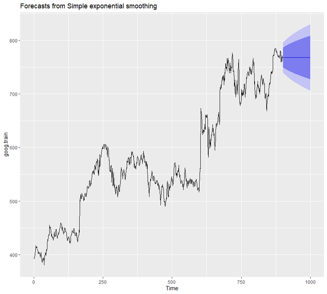
从上面的输出图中，我们可以注意到我们的预测模型对未来的预测是扁平的。因此，我们可以说，从数据来看，它没有捕捉到当前的趋势。因此，为了纠正这个问题，我们将使用diff()函数从数据中删除趋势。

示例 2：

R

# SES in R
# loading the required packages
library(tidyverse)
library(fpp2)
 
# create training and validation
# of the Google stock data
goog.train <- window(goog,
                     end = 900)
goog.test <- window(goog,
                    start = 901)
 
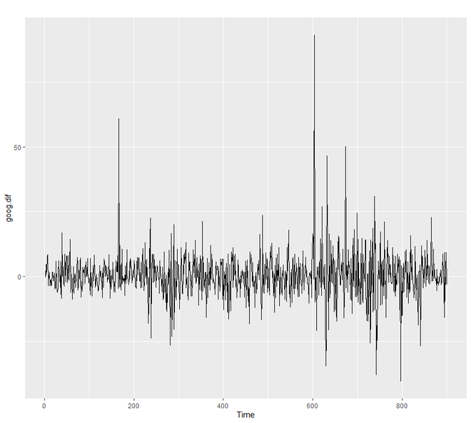
# removing the trend
goog.dif <- diff(goog.train)
autoplot(goog.dif)
 
# reapplying SES on the filtered data
ses.goog.dif <- ses(goog.dif,
                    alpha = .2,
                    h = 100)
autoplot(ses.goog.dif)

输出：

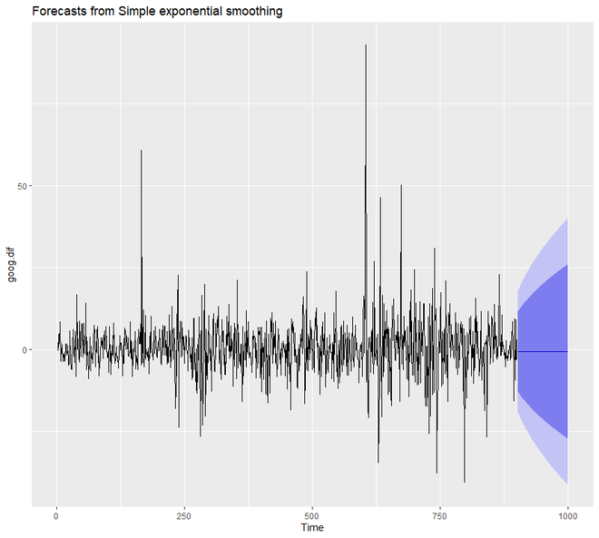
为了了解我们模型的性能，我们需要将我们的预测与我们的验证或测试数据集进行比较。由于我们的训练数据集是不同的，我们也需要形成或创建不同的验证或测试集。

示例 3：

在这里，我们将创建一个差异验证集，然后将我们的预测与验证集进行比较。在这里，我们使用循环将 alpha 的值设置为 0.01-0.99。我们正在尝试了解哪个级别将最小化 RMSE 测试。我们将看到 0.05 将最小化。

R

# SES in R
# loading the required packages
library(tidyverse)
library(fpp2)
 
# create training and validation
# of the Google stock data
goog.train <- window(goog,
                     end = 900)
goog.test <- window(goog,
                    start = 901)
 
# removing trend from test set
goog.dif.test <- diff(goog.test)
accuracy(ses.goog.dif, goog.dif.test)
 
# comparing our model
alpha <- seq(.01, .99, by = .01)
RMSE <- NA
for(i in seq_along(alpha)) {
  fit <- ses(goog.dif, alpha = alpha[i],
             h = 100)
  RMSE[i] <- accuracy(fit,
                      goog.dif.test)[2,2]
}
 
# convert to a data frame and
# identify min alpha value
alpha.fit <- data_frame(alpha, RMSE)
alpha.min <- filter(alpha.fit,
                    RMSE == min(RMSE))
 
# plot RMSE vs. alpha
ggplot(alpha.fit, aes(alpha, RMSE)) +
  geom_line() +
  geom_point(data = alpha.min,
             aes(alpha, RMSE),
             size = 2, color = "red")

输出：

ME     RMSE      MAE       MPE     MAPE      MASE        ACF1 Theil's U
Training set -0.01368221 9.317223 6.398819  99.97907 253.7069 0.7572009 -0.05440377        NA
Test set      0.97219517 8.141450 6.117483 109.93320 177.9684 0.7239091  0.12278141 0.9900678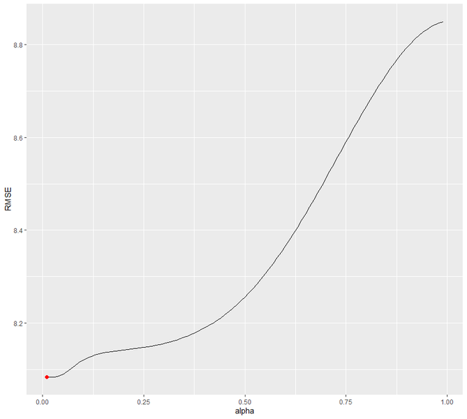

现在，我们将尝试重新拟合 alpha =0.05 的 SES 预测模型。我们会注意到 alpha 0.02 和 alpha=0.05 之间的显着差异。

示例 4：

R

# SES in R
# loading packages
library(tidyverse)
library(fpp2)
 
# create training and validation
# of the Google stock data
goog.train <- window(goog,
                     end = 900)
goog.test <- window(goog,
                    start = 901)
 
# removing trend
goog.dif <- diff(goog.train)
 
# refit model with alpha = .05
ses.goog.opt <- ses(goog.dif,
                    alpha = .05,
                    h = 100)
 
# performance eval
accuracy(ses.goog.opt, goog.dif.test)
 
# plotting results
p1 <- autoplot(ses.goog.opt) +
  theme(legend.position = "bottom")
p2 <- autoplot(goog.dif.test) +
  autolayer(ses.goog.opt, alpha = .5) +
  ggtitle("Predicted vs. actuals for
                 the test data set")
 
gridExtra::grid.arrange(p1, p2,
                        nrow = 1)

输出：

> accuracy(ses.goog.opt, goog.dif.test)
                      ME     RMSE      MAE       MPE     MAPE      MASE       ACF1 Theil's U
Training set -0.01188991 8.939340 6.030873 109.97354 155.7700 0.7136602 0.01387261        NA
Test set      0.30483955 8.088941 6.028383  97.77722 112.2178 0.7133655 0.12278141 0.9998811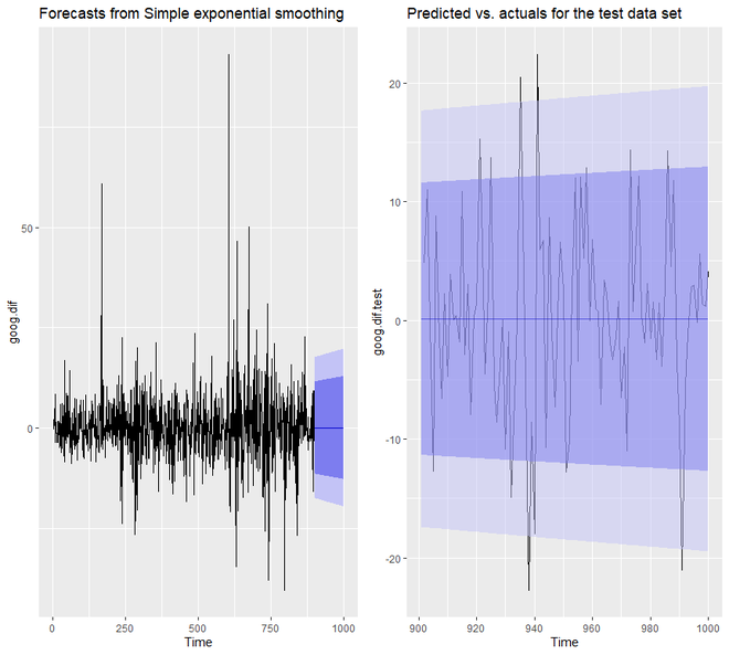

我们将看到，现在我们模型的预测置信区间要窄得多。

霍尔特方法

我们已经看到，在 SES 中，我们必须删除长期趋势来改进模型。但是在Holt 方法中，我们可以在捕捉数据趋势的同时应用指数平滑。这是一种适用于具有趋势但没有季节性的数据的技术。为了对数据进行预测，Holt 方法使用两个平滑参数 alpha和 beta ，它们对应于水平分量和趋势分量。

在 R 中，为了应用 Holt 方法，我们将使用holt()函数。我们将再次通过一些示例来了解该技术的工作原理。我们将再次使用 goog 数据集。

示例 1：

R

# holt's method in R
 
# loading packages
library(tidyverse)
library(fpp2)
 
# create training and validation
# of the Google stock data
goog.train <- window(goog,
                     end = 900)
goog.test <- window(goog,
                    start = 901)
 
# applying holt's method on
# Google stock Data
holt.goog <- holt(goog.train,
                  h = 100)
autoplot(holt.goog)

输出：

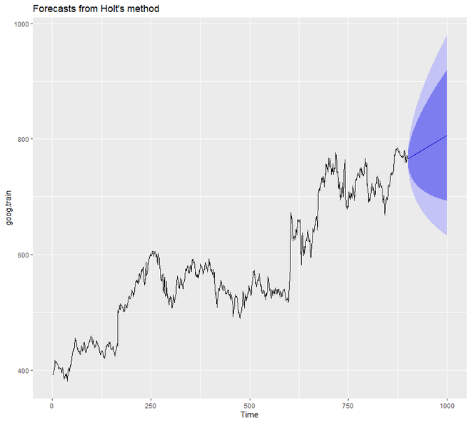
在上面的例子中，我们没有手动设置 alpha 和 beta 的值。但我们可以这样做。但是，如果我们确实提到了 alpha 和 beta 的任何值，那么holt()函数将自动识别最佳值。在这种情况下，如果 alpha 的值为 0.9967，则表明学习速度快，如果 beta 的值为 0.0001，则表明趋势学习缓慢。

示例 2：

在本例中，我们将设置 alpha 和 beta 的值。此外，我们将看到模型的准确性。

R

# holt's method in R
 
# loading the packages
library(tidyverse)
library(fpp2)
 
# create training and validation
# of the Google stock data
goog.train <- window(goog,
                     end = 900)
goog.test <- window(goog,
                    start = 901)
 
# holt's method
holt.goog$model
 
# accuracy of the model
accuracy(holt.goog, goog.test)

输出：

Holt's method 

Call:
 holt(y = goog.train, h = 100) 

  Smoothing parameters:
    alpha = 0.9999 
    beta  = 1e-04 

  Initial states:
    l = 401.1276 
    b = 0.4091 

  sigma:  8.8149

     AIC     AICc      BIC 
10045.74 10045.81 10069.75 

> accuracy(holt.goog, goog.test)
                       ME      RMSE       MAE         MPE     MAPE     MASE       ACF1 Theil's U
Training set -0.003332796  8.795267  5.821057 -0.01211821 1.000720 1.002452 0.03100836        NA
Test set      0.545744415 16.328680 12.876836  0.03013427 1.646261 2.217538 0.87733298  2.024518

最优值即 beta = 0.0001 用于从训练集中去除错误。我们可以将我们的 beta 调整到这个最佳值。

示例 3：

让我们试着找到 beta 的最优值 通过一个范围从 0.0001 到 0.5 的循环，这将最小化 RMSE 测试。我们将看到 0.0601 将是使 RMSE 下降的 beta 值。

R

# holts method in R
# loading the package
library(tidyverse)
library(fpp2)
 
# create training and validation
# of the Google stock data
goog.train <- window(goog,
                     end = 900)
goog.test <- window(goog,
                    start = 901)
 
# identify optimal alpha parameter
beta <- seq(.0001, .5, by = .001)
RMSE <- NA
for(i in seq_along(beta)) {
  fit <- holt(goog.train,
              beta = beta[i],
              h = 100)
  RMSE[i] <- accuracy(fit,
                      goog.test)[2,2]
}
 
# convert to a data frame and
# identify min alpha value
beta.fit <- data_frame(beta, RMSE)
beta.min <- filter(beta.fit,
                   RMSE == min(RMSE))
 
# plot RMSE vs. alpha
ggplot(beta.fit, aes(beta, RMSE)) +
  geom_line() +
  geom_point(data = beta.min,
             aes(beta, RMSE),
             size = 2, color = "red")

输出：

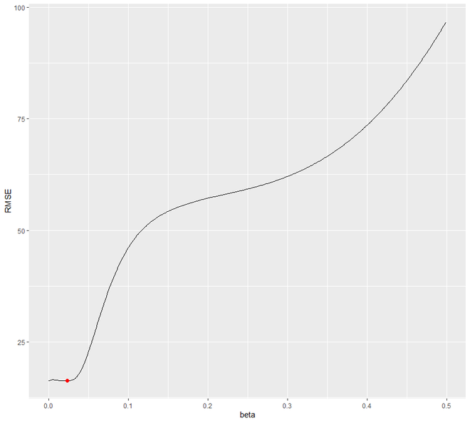
现在让我们用获得的最佳 beta 值重新拟合模型。

示例 4：

我们将设置 beta nad 的最佳值，并将预测准确性与我们的原始模型进行比较。

R

# loading the package
library(tidyverse)
library(fpp2)
 
# create training and validation
# of the Google stock data
goog.train <- window(goog,
                     end = 900)
goog.test <- window(goog,
                    start = 901)
 
holt.goog <- holt(goog.train,
                  h = 100)
 
# new model with optimal beta
holt.goog.opt <- holt(goog.train,
                      h = 100,
                      beta = 0.0601)
 
# accuracy of first model
accuracy(holt.goog, goog.test)
 
# accuracy of new optimal model
accuracy(holt.goog.opt, goog.test)
 
p1 <- autoplot(holt.goog) +
  ggtitle("Original Holt's Model") +
  coord_cartesian(ylim = c(400, 1000))
 
p2 <- autoplot(holt.goog.opt) +
  ggtitle("Optimal Holt's Model") +
  coord_cartesian(ylim = c(400, 1000))
 
gridExtra::grid.arrange(p1, p2,
                        nrow = 1)

输出：

> accuracy(holt.goog, goog.test)
                       ME      RMSE       MAE         MPE     MAPE     MASE       ACF1 Theil's U
Training set -0.003332796  8.795267  5.821057 -0.01211821 1.000720 1.002452 0.03100836        NA
Test set      0.545744415 16.328680 12.876836  0.03013427 1.646261 2.217538 0.87733298  2.024518

> accuracy(holt.goog.opt, goog.test)
                      ME      RMSE       MAE          MPE     MAPE     MASE        ACF1 Theil's U
Training set -0.01493114  8.960214  6.058869 -0.005524151 1.039572 1.043406 0.009696325        NA
Test set     21.41138275 28.549029 23.841097  2.665066997 2.988712 4.105709 0.895371665  3.435763

我们会注意到，与原始模型相比，最优模型要保守得多。此外，最优模型的置信区间更加极端。

Holt-Winter 的季节性方法

Holt-Winter 的季节性方法用于具有季节性模式和趋势的数据。此方法可以通过使用加法结构或乘法结构来实现，具体取决于数据集。当数据的季节性模式具有相同的幅度或始终一致时，使用加法结构或模型，而如果数据的季节性模式的幅度随时间增加，则使用乘法结构或模型。它使用三个平滑参数 - alpha、beta 和 gamma 。

在 R 中，我们使用decompose()函数来执行这种指数平滑。我们将使用 qcement 数据集来研究这种技术的工作原理。

示例 1：

R

# Holt-Winter's method in R
# loading packages
library(tidyverse)
library(fpp2)
 
# create training and validation
# of the AirPassengers data
qcement.train <- window(qcement,
                        end = c(2012, 4))
qcement.test <- window(qcement,
                       start = c(2013, 1))
 
# applying holt-winters
# method on qcement
autoplot(decompose(qcement))

输出：

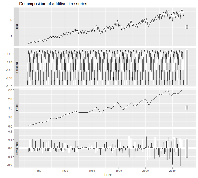
为了创建一个处理误差、趋势和季节性的加法模型，我们将使用ets()函数。在 36 个模型中， ets()选择了最佳的加法模型。对于加法模型， ets()的模型参数将为“AAA”。

示例 2：

R

# loading package
library(tidyverse)
library(fpp2)
 
# create training and validation
# of the AirPassengers data
qcement.train <- window(qcement,
                        end = c(2012, 4))
qcement.test <- window(qcement,
                       start = c(2013, 1))
 
# applying ets
qcement.hw <- ets(qcement.train,
                  model = "AAA")
autoplot(forecast(qcement.hw))

输出：

现在我们将评估我们的模型并总结平滑参数。我们还将检查残差并找出我们模型的准确性。

示例 3：

R

# additive model
# loading packages
library(tidyverse)
library(fpp2)
 
# create training and validation
# of the AirPassengers data
qcement.train <- window(qcement,
                        end = c(2012, 4))
qcement.test <- window(qcement,
                       start = c(2013, 1))
 
qcement.hw <- ets(qcement.train, model = "AAA")
 
# assessing our model
summary(qcement.hw)
checkresiduals(qcement.hw)
 
# forecast the next 5 quarters
qcement.f1 <- forecast(qcement.hw,
                       h = 5)
 
# check accuracy
accuracy(qcement.f1, qcement.test)

输出：

> summary(qcement.hw)
ETS(A,A,A) 

Call:
 ets(y = qcement.train, model = "AAA") 

  Smoothing parameters:
    alpha = 0.6418 
    beta  = 1e-04 
    gamma = 0.1988 

  Initial states:
    l = 0.4511 
    b = 0.0075 
    s = 0.0049 0.0307 9e-04 -0.0365

  sigma:  0.0854

     AIC     AICc      BIC 
126.0419 126.8676 156.9060 

Training set error measures:
                      ME       RMSE       MAE          MPE     MAPE      MASE       ACF1
Training set 0.001463693 0.08393279 0.0597683 -0.003454533 3.922727 0.5912949 0.02150539

> checkresiduals(qcement.hw)

    Ljung-Box test

data:  Residuals from ETS(A,A,A)
Q* = 20.288, df = 3, p-value = 0.0001479

Model df: 8.   Total lags used: 11

> accuracy(qcement.f1, qcement.test)
                      ME       RMSE        MAE          MPE     MAPE      MASE        ACF1 Theil's U
Training set 0.001463693 0.08393279 0.05976830 -0.003454533 3.922727 0.5912949  0.02150539        NA
Test set     0.031362775 0.07144211 0.06791904  1.115342984 2.899446 0.6719311 -0.31290496 0.2112428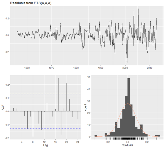

现在我们将看到乘法模型如何使用ets()工作。为此， ets()的模型参数将是“MAM”。

示例 4：

R

# multiplicative model in R
# loading package
library(tidyverse)
library(fpp2)
 
# create training and validation
# of the AirPassengers data
qcement.train <- window(qcement,
                        end = c(2012, 4))
qcement.test <- window(qcement,
                       start = c(2013, 1))
 
# applying ets
qcement.hw2 <- ets(qcement.train,
                   model = "MAM")
checkresiduals(qcement.hw2)

输出：

> checkresiduals(qcement.hw2)

    Ljung-Box test

data:  Residuals from ETS(M,A,M)
Q* = 23.433, df = 3, p-value = 3.281e-05

Model df: 8.   Total lags used: 11

在这里，我们将优化 gamma 参数以最小化错误率。 gamma 的值为 0.21。除此之外，我们将找出准确性并绘制预测值。

示例 5：

R

# Holt winters model in R
# loading packages
library(tidyverse)
library(fpp2)
 
# create training and validation
# of the AirPassengers data
qcement.train <- window(qcement,
                        end = c(2012, 4))
qcement.test <- window(qcement,
                       start = c(2013, 1))
 
qcement.hw <- ets(qcement.train,
                  model = "AAA")
 
# forecast the next 5 quarters
qcement.f1 <- forecast(qcement.hw,
                       h = 5)
 
# check accuracy
accuracy(qcement.f1, qcement.test)
 
gamma <- seq(0.01, 0.85, 0.01)
RMSE <- NA
 
for(i in seq_along(gamma)) {
  hw.expo <- ets(qcement.train,
                 "AAA",
                 gamma = gamma[i])
  future <- forecast(hw.expo,
                     h = 5)
  RMSE[i] = accuracy(future,
                     qcement.test)[2,2]
}
 
error <- data_frame(gamma, RMSE)
minimum <- filter(error,
                  RMSE == min(RMSE))
ggplot(error, aes(gamma, RMSE)) +
  geom_line() +
  geom_point(data = minimum,
             color = "blue", size = 2) +
  ggtitle("gamma's impact on
            forecast errors",
  subtitle = "gamma = 0.21 minimizes RMSE")
 
# previous model with additive
# error, trend and seasonality
accuracy(qcement.f1, qcement.test)
 
 
# new model with
# optimal gamma parameter
qcement.hw6 <- ets(qcement.train,
                   model = "AAA",
                   gamma = 0.21)
qcement.f6 <- forecast(qcement.hw6,
                       h = 5)
accuracy(qcement.f6, qcement.test)
 
# predicted values
qcement.f6
autoplot(qcement.f6)

输出：

> accuracy(qcement.f1, qcement.test)
                      ME       RMSE        MAE          MPE     MAPE      MASE        ACF1 Theil's U
Training set 0.001463693 0.08393279 0.05976830 -0.003454533 3.922727 0.5912949  0.02150539        NA
Test set     0.031362775 0.07144211 0.06791904  1.115342984 2.899446 0.6719311 -0.31290496 0.2112428

> accuracy(qcement.f6, qcement.test)
                       ME       RMSE        MAE        MPE     MAPE      MASE        ACF1 Theil's U
Training set -0.001312025 0.08377557 0.05905971 -0.2684606 3.834134 0.5842847  0.04832198        NA
Test set      0.033492771 0.07148708 0.06775269  1.2096488 2.881680 0.6702854 -0.35877010 0.2202448

> qcement.f6
        Point Forecast    Lo 80    Hi 80    Lo 95    Hi 95
2013 Q1       2.134650 2.025352 2.243947 1.967494 2.301806
2013 Q2       2.427828 2.299602 2.556055 2.231723 2.623934
2013 Q3       2.601989 2.457284 2.746694 2.380681 2.823296
2013 Q4       2.505001 2.345506 2.664496 2.261075 2.748927
2014 Q1       2.171068 1.987914 2.354223 1.890958 2.451179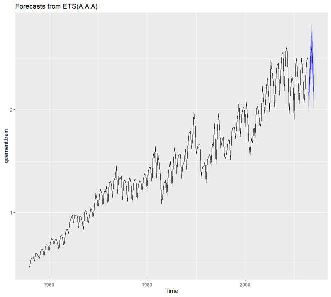

R中的阻尼方法

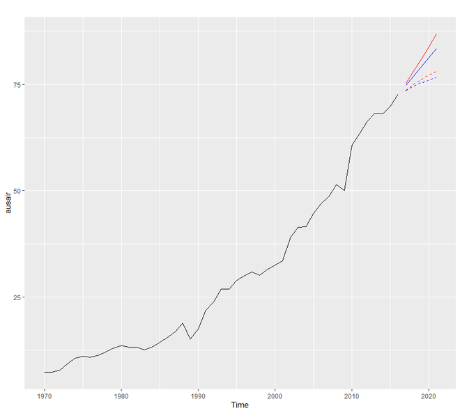
阻尼方法使用阻尼系数 phi来更保守地估计预测趋势。 phi 的值介于 0 和 1 之间。如果我们相信我们的加法和乘法模型将是一条平线，那么它就有可能是阻尼的。为了理解阻尼预测的工作原理，我们将使用fpp2::ausair数据集，我们将在其中创建许多模型并尝试使用更保守的趋势线，

例子：

R

# Damping model in R
 
# loading the packages
library(tidyverse)
library(fpp2)
 
# holt's linear (additive) model
fit1 <- ets(ausair, model = "ZAN",
            alpha = 0.8, beta = 0.2)
pred1 <- forecast(fit1, h = 5)
 
# holt's linear (additive) model
fit2 <- ets(ausair, model = "ZAN",
            damped = TRUE, alpha = 0.8,
            beta = 0.2, phi = 0.85)
pred2 <- forecast(fit2, h = 5)
 
# holt's exponential
# (multiplicative) model
fit3 <- ets(ausair, model = "ZMN",
            alpha = 0.8, beta = 0.2)
pred3 <- forecast(fit3, h = 5)
 
# holt's exponential
# (multiplicative) model damped
fit4 <- ets(ausair, model = "ZMN",
            damped = TRUE,
            alpha = 0.8, beta = 0.2,
            phi = 0.85)
pred4 <- forecast(fit4, h = 5)
 
autoplot(ausair) +
  autolayer(pred1$mean,
            color = "blue") +
  autolayer(pred2$mean,
            color = "blue",
            linetype = "dashed") +
  autolayer(pred3$mean,
            color = "red") +
  autolayer(pred4$mean,
            color = "red",
            linetype = "dashed")

输出：