使用 R 编程进行主成分分析

R编程中的主成分分析（PCA） 是对所有现有属性的线性分量的分析。主成分是数据集中原始预测变量的线性组合（正交变换）。它是 EDA（探索性数据分析）的一种有用技术，可让您更好地可视化具有许多变量的数据集中存在的变化。

R – 主成分分析

第一个主成分捕获数据集中的最大方差。它决定了更高可变性的方向。第二个主成分捕获数据中的剩余方差，并且与 PC1 不相关。 PC1 和 PC2 之间的相关性应该为零。因此，所有后续的主成分都遵循相同的概念。它们捕获剩余的方差，而不与之前的主成分相关。

数据集

数据集mtcars （电机趋势汽车道路测试）包括 32 辆汽车的油耗和汽车设计和性能的 10 个方面。它预装了 R 中的 dplyr 包。

R

# Installing required package
install.packages("dplyr")
 
# Loading the package
library(dplyr)
 
# Importing excel file
str(mtcars)

输出：

使用 R 语言使用数据集进行主成分分析

我们对包含 32 个汽车品牌和 10 个变量的mtcars进行主成分分析。

R

# Loading Data
data(mtcars)
 
# Apply PCA using prcomp function
# Need to scale / Normalize as
# PCA depends on distance measure
my_pca <- prcomp(mtcars, scale = TRUE,
                center = TRUE, retx = T)
names(my_pca)
 
# Summary
summary(my_pca)
my_pca
 
# View the principal component loading
# my_pca$rotation[1:5, 1:4]
my_pca$rotation
 
# See the principal components
dim(my_pca$x)
my_pca$x
 
# Plotting the resultant principal components
# The parameter scale = 0 ensures that arrows
# are scaled to represent the loadings
biplot(my_pca, main = "Biplot", scale = 0)
 
# Compute standard deviation
my_pca$sdev
 
# Compute variance
my_pca.var <- my_pca$sdev ^ 2
my_pca.var
 
# Proportion of variance for a scree plot
propve <- my_pca.var / sum(my_pca.var)
propve
 
# Plot variance explained for each principal component
plot(propve, xlab = "principal component",
            ylab = "Proportion of Variance Explained",
            ylim = c(0, 1), type = "b",
            main = "Scree Plot")
 
# Plot the cumulative proportion of variance explained
plot(cumsum(propve),
    xlab = "Principal Component",
    ylab = "Cumulative Proportion of Variance Explained",
    ylim = c(0, 1), type = "b")
 
# Find Top n principal component
# which will atleast cover 90 % variance of dimension
which(cumsum(propve) >= 0.9)[1]
 
# Predict mpg using first 4 new Principal Components
# Add a training set with principal components
train.data <- data.frame(disp = mtcars$disp, my_pca$x[, 1:4])
 
# Running a Decision tree algporithm
## Installing and loading packages
install.packages("rpart")
install.packages("rpart.plot")
library(rpart)
library(rpart.plot)
 
rpart.model <- rpart(disp ~ .,
                    data = train.data, method = "anova")
 
rpart.plot(rpart.model)

输出：

• 毕情节

• 生成的主成分绘制为Biplot 。比例值 0 表示箭头按比例表示载荷。
• 解释每个主成分的方差

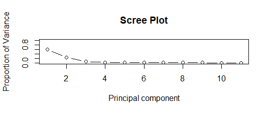
• 碎石图表示方差和主成分的比例。在 2 个主成分以下，有一个最大比例的方差，如图所示。
• 累计方差比例

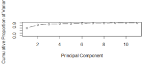
• 碎石图表示方差和主成分的累积比例。在 2 个主成分之上，有一个最大的累积方差比例，如图所示。
• 决策树模型

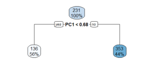
• 建立决策树模型以使用数据集中的其他变量和使用 ANOVA 方法来预测disp 。绘制决策树图并显示信息。