使用 ColumnTransformer、OneHotEncoder 和 Pipeline 进行预测

在本教程中，我们将使用 ColumnTransformer、OneHotEncoder 和 Pipeline 预测每个具有各种功能的客户的保险费成本。
我们将导入必要的数据操作库：
代码：

import pandas as pd
import numpy as np
  
from sklearn.compose import ColumnTransformer
from sklearn.model_selection import train_test_split, cross_val_score
from sklearn.impute import SimpleImputer
from sklearn.preprocessing import OneHotEncoder, StandardScaler, MinMaxScaler
from sklearn.pipeline import Pipeline
from sklearn.ensemble import RandomForestRegressor

我们现在将加载数据集，可在此处获得：
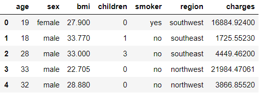
每行是一个不同的人，有年龄、性别、体重指数 (bmi)、家属人数、是否吸烟、所属地区以及他们支付的保险费。

代码：

df = pd.read_csv('https://raw.githubusercontent.com / stedy / Machine-Learning-with-R-datasets / master / insurance.csv')
df.head()

代码：

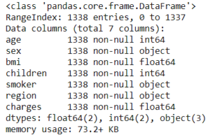
df.info()

代码：

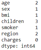
df.isna().sum()

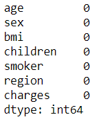
我们看到没有。但是我们将在这个数据集中引入“杂质”，因为平静的大海从来没有造就过熟练的水手！ …除了我们需要缺失值来以更好的方式演示 ColumnTransformer 之外。

代码：

np.random.seed(0) # for reproducibility
for _ in range(10):
    r = np.random.randint(len(df))
    c = np.random.randint(6)
    df.iloc[r, c] = np.nan

对于 range(10)，我们暗示我们需要在数据中的 10 个位置使用 NaN，无论是不同行中的每个 NaN 还是一行中的多个 NaN，我们都不会介意。

代码：

df.isna().sum()

我们现在将数据分成训练集和测试集。

代码：

X_train, X_test, y_train, y_test = train_test_split(df.drop('charges', 1),
                                                    df['charges'],
                                                    test_size = 0.2, random_state = 0)

现在进入 ColumnTransformer！
ColumnTransformer 接受一个列表，其中包含我们希望在不同列上执行的转换的元组。每个元组需要 3 个逗号分隔的值：首先，转换器的名称，实际上可以是任何东西（作为字符串传递），第二个是估计器对象，最后一个是我们希望执行该操作的列.

代码：

trf1 = ColumnTransformer(transformers =[
    ('cat', SimpleImputer(strategy ='most_frequent'), ['sex', 'smoker', 'region']),
    ('num', SimpleImputer(strategy ='median'), ['age', 'bmi', 'children']),
      
], remainder ='passthrough')

首先，我们将估算分类列。我们将使用 most_frequent 或“mode”类型的插补，分类列是“sex”、“smoker”和“region”。为简单起见，我们将这个转换器命名为“猫”。
同样，我们将使用各个列的中位数对数值列进行插补。我们现在需要告诉 ColumnTransformer 它应该如何处理剩余的列，即没有执行转换的列。在我们的例子中，所有功能都被使用，但如果您有“未使用”的列，您可以指定在转换后是要删除还是保留这些列。我们将保留它们，因此传递剩余='passthrough' 而不是删除这些列的默认行为。我们也可以将列指定为整数位置而不是名称，例如 ['age', 'bmi', 'children']，我们可以说 [0, 2, 3] 等。现在我们将拟合并转换 X_train 以查看输出，默认情况下是一个 numpy 数组：
代码：

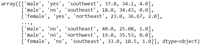
first_step = trf1.fit_transform(X_train)
first_step

我们将用它制作一个数据框：
代码：

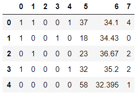
pd.DataFrame(first_step).head()

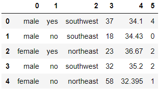
您是否注意到列已重新排序，并且列名现在丢失了？它们已按照我们传递给 ColumnTransformer 的转换器的顺序重新排序，即我们首先要求它估算分类列，因此它们被放在首位，依此类推……

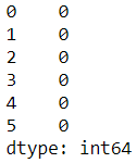
代码：

pd.DataFrame(first_step).isna().sum()

我们可以通过使用我们在元组中传递的“名称”来检查每个转换器正在做什么：
代码：

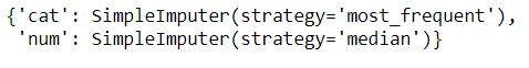
trf1.named_transformers_
# this is a dictionary, with the names of the transformers as keys.

代码：

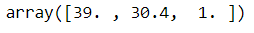
trf1.named_transformers_['num'].statistics_
# you see, these were the median values of each of the three numerical columns.
# for any transformer, you can access its specific attributes this way.

现在所有列都没有缺失值，我们可以继续对分类列进行编码。

注意：OneHotEncoder 无法处理缺失值，因此在编码之前删除它们很重要。现在，我们为编码制作另一个转换器对象。我们无法在 'trf1' 中执行此操作，因为在那个时间点，X_train 中存在缺失值，并且 OneHotEncoder 无法处理前面讨论的缺失值。因此，我们首先需要删除缺失值，然后将这个新的“first_step”数组（没有缺失值）传递给 OneHotEncoder。

代码：

trf2 = ColumnTransformer(transformers =[
    ('enc', OneHotEncoder(sparse = False, drop ='first'), list(range(3))),
], remainder ='passthrough')

我们将 sparse 参数设置为 False（因为我们想要一个密集的数组输出），并且我们可以在删除第一个虚拟编码列之间切换，这取决于我们拟合的模型的类型，以避免“虚拟变量陷阱” '。在此处了解更多信息：一般经验法则：如果使用基于线性的模型，则删除一个虚拟编码列，如果使用基于树的模型，则不要删除它。另外，您是否看到对于 columns 参数，我们如何指定list(range(3))而不是列名？那是因为现在，我们丢失了列名（如“first_step”中所示，但我们知道分类列是前三列（重新排序后），因此我们指定 [0, 1, 2]。

代码：

second_step = trf2.fit_transform(first_step)
pd.DataFrame(second_step).head()
  
# Now we have our one hot encoded data ! Sweet !

现在来了管道！我们可以在一个 Pipeline 实例中执行所有这些步骤。管道还需要一个元组列表，每个元组又需要两个值：步骤名称和对象。

代码：

pipe = Pipeline(steps =[
    ('tf1', trf1),
    ('tf2', trf2),
    ('tf3', MinMaxScaler()), # or StandardScaler, or any other scaler
    ('model', RandomForestRegressor(n_estimators = 200)),
# or LinearRegression, SVR, DecisionTreeRegressor, etc
])

代码：

# we'll use cross_val_score with 5 splits to better examine our model.
# we'll send our entire 'pipe' object to the cross_val_score and it will take
# care of all the preprocessing work for us ! cvs = cross_val_score(pipe, X_train, y_train, cv = 5)
print("All cross val scores:", cvs)
print("Mean of all scores: ", cvs.mean())

所以我们的模型准确率约为 81.2%。您可以尝试不同的回归器、调整参数、使用 StandardScaler 或其他缩放器，看看是否可以获得更好的结果。我们可以使用 GridSearchCV 来完成这项为我们寻找最佳参数集的工作。我们现在将在整个训练集上拟合模型，并在测试集上预测结果：

代码：

pipe.fit(X_train, y_train)

代码：

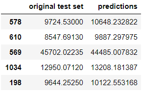
preds = pipe.predict(X_test)
  
# This is how the original test set insurance prices and 
# our predicted ones stack up
  
pd.DataFrame({'original test set':y_test, 'predictions': preds})