使用 R 编程的 Bootstrap 置信区间

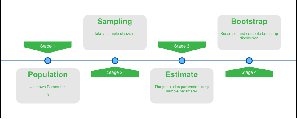
Bootstrapping 是一种使用样本数据推断总体的统计方法。它可用于通过从样本数据中抽取带有替换的样本来估计置信区间 (CI)。 Bootstrapping 可用于将 CI 分配给没有封闭形式或复杂解决方案的各种统计信息。假设我们要使用自举重采样获得 95% 的置信区间，步骤如下：

1. 从原始样本数据中对 n 个元素进行替换。
2. 对于每个样本，计算所需的统计数据，例如。平均值、中位数等
3. 重复步骤 1 和 2 m 次并保存计算的统计信息。
4. 绘制形成引导分布的计算统计数据
5. 使用所需统计数据的引导分布，我们可以计算 95% CI

从样本中生成引导分布的图示：

R中的实现

在 R Programming 中，包引导允许用户轻松生成几乎任何我们可以计算的统计数据的引导样本。我们可以从引导包的计算中生成偏差估计、引导置信区间或引导分布图。

出于演示目的，我们将使用鸢尾花数据集作为 R 中的内置数据集之一，因为它的简单性和可用性。该数据集由来自三种鸢尾花（Iris setosa，Iris Virginia）中的每一种的 50 个样本组成。和虹膜）。从每个样本中测量了四个特征：萼片和花瓣的长度和宽度，以厘米为单位。我们可以使用 head 命令查看 iris 数据集并注意感兴趣的特征。

R

# View the first row
# of the iris dataset
head(iris, 1)

输出：

Sepal.Length    Sepal.Width    Petal.Length    Petal.Width    Species
     5.1             3.5              1.4             0.2      setosa

我们想估计花瓣长度和花瓣宽度之间的相关性。

在 R 中计算 Bootstrap CI 的步骤：

1.导入boot库计算bootstrap CI和ggplot2作图。

R

# Import library for bootstrap methods
library(boot)
 
# Import library for plotting
library(ggplot2)

2. 创建一个函数来计算我们想要使用的统计量，例如平均值、中位数、相关性等。

R

# Custom function to find correlation
# between the Petal Length and Width
corr.fun <- function(data, idx)
{
  df <- data[idx, ]
 
  # Find the spearman correlation between
  # the 3rd and 4th columns of dataset
  c(cor(df[, 3], df[, 4], method = 'spearman'))
}

3. 使用boot函数求统计量的R bootstrap。

R

# Setting the seed for
# reproducability of results
set.seed(42)
 
# Calling the boot function with the dataset
# our function and no. of rounds
bootstrap <- boot(iris, corr.fun, R = 1000)
 
# Display the result of boot function
bootstrap

输出：

ORDINARY NONPARAMETRIC BOOTSTRAP


Call:
boot(data = iris, statistic = corr.fun, R = 1000)


Bootstrap Statistics :
     original       bias    std. error
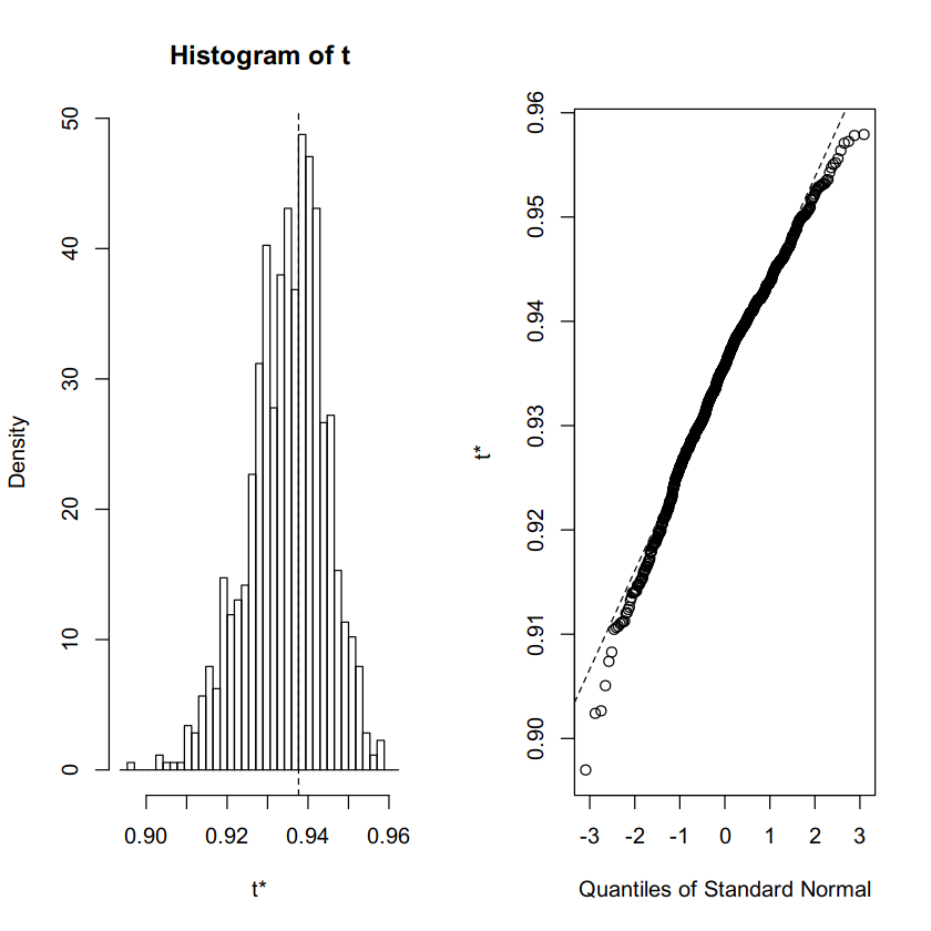
t1* 0.9376668 -0.002717295 0.009436212

4. 我们可以使用带有计算引导程序的 plot 命令绘制生成的引导程序分布。

R

# Plot the bootstrap sampling
# distribution using ggplot
plot(bootstrap)

输出：

5. 使用boot.ci()函数获取置信区间。

R

# Function to find the
# bootstrap Confidence Intervals
boot.ci(boot.out = bootstrap,
        type = c("norm", "basic",
                 "perc", "bca"))

输出：

BOOTSTRAP CONFIDENCE INTERVAL CALCULATIONS
Based on 1000 bootstrap replicates

CALL : 
boot.ci(boot.out = bootstrap, type = c("norm", "basic", "perc", 
    "bca"))

Intervals : 
Level      Normal              Basic         
95%   ( 0.9219,  0.9589 )   ( 0.9235,  0.9611 )  

Level     Percentile            BCa          
95%   ( 0.9142,  0.9519 )   ( 0.9178,  0.9535 )  
Calculations and Intervals on Original Scale

从输出推断 Bootstrap CI：

查看 (0.9219, 0.9589) 的 Normal 方法区间，我们可以 95% 确定花瓣长度和宽度之间的实际相关性在 95% 的时间中位于该区间。正如我们所见，输出由多个 CI 组成，根据函数boot.ci 中的类型参数使用不同的方法。计算的区间对应于（“norm”、“basic”、“perc”、“bca”）或 Normal、Basic、Percentile 和 BCa，它们为相同的 95% 水平提供不同的区间。用于任何变量的具体方法取决于各种因素，例如其分布、同方差、偏差等。

下面总结了引导包为引导置信区间提供的 5 种方法：

1. 正态自举或标准置信限方法使用标准偏差来计算 CI。
   • 在统计数据无偏时使用。
   • 是正态分布的。
2. 基本自举或霍尔（第二个百分位）方法使用百分位计算检验统计量的上限和下限。
   • 当统计数据是无偏且同方差的。
   • 引导统计量可以转换为标准正态分布。
3. Percentile bootstrap或 Quantile-based，或 Approximate 间隔使用分位数，例如 2.5%、5% 等来计算 CI。
   • 当统计数据无偏且均方差时使用。
   • 您的引导统计量和样本统计量的标准误差是相同的。
4. BCa bootstrap或 Bias Corrected Accelerated 使用带有偏差校正的百分位限制和估计加速度系数来校正限制并找到 CI。
   • 引导统计量可以转换为正态分布。
   • 正态变换的统计量具有恒定的偏差。
5. Studentized bootstrap对 bootstrap 样本进行重新采样，以找到第二阶段的 bootstrap 统计量并使用它来计算 CI。
   • 当统计量是同方差时使用。
   • 引导统计量的标准误差可以通过第二阶段重采样来估计。

参考 ：
R 引导程序包引导
自举统计维基百科
置信区间的引导程序