Gibb's Phenomenon Rectangular 和 Hamming Window 实现

Gibb's Phenomenon Rectangular 和 Hamming Window 实现

什么是吉布现象？

数字滤波器中的吉布现象是指周期函数的傅立叶级数在跳跃中断附近的行为方式，傅立叶级数的部分和在中断附近有很大的振荡，这可能会使部分和的最大值增加到函数本身的最大值之上.因此，当傅立叶级数在不连续点处添加项时，会出现过冲。

在信号处理方面，我们可以将吉布现象转化为滤波器的阶跃响应，通过傅立叶级数截断我们的信号可以称为滤除信号。

我们将通过示例问题来理解这一点：

过滤器规格

1. 具有 41 个抽头的数字低通 FIR 滤波器。
2. 滤波器的截止频率为 pi/4

我们将同时使用矩形和汉明窗技术来实施该解决方案。

什么是矩形窗技术？

在矩形窗口中，傅立叶变换收敛到sinc函数，在边缘给出矩形形状，因此名称为矩形窗口。矩形在工业中并未广泛用于过滤信号。

什么是汉明窗技术？

汉明窗是一种更优化的信号滤波方法，因为它切断了任一侧的信号点，让我们可以更清晰地看到信号频谱。

循序渐进的方法：

第 1 步：导入所有必要的库。

Python3

##import required library
import numpy as np
import scipy.signal as signal
import matplotlib.pyplot as plt

第 2 步：使用给定的过滤器规格定义变量。

蟒蛇3

#Given specification
wc =np.pi/4        #Cutoff frequency in radian
N1=int(input())    #Given filter length
M=(N1-1)/2         #Half length of the filter

步骤 3：计算幅度、相位响应以获得矩形窗口系数

蟒蛇3

N = 512    ## Choose DFT size
n = np.arange(-M,M)  
#Desired impulse response coefficients of the lowpass
#filter with cutoff frequency wc
hd = wc / np.pi * np.sinc(wc * (n) / np.pi)
 
#Select the rectangular window coefficients
win =signal.boxcar(len(n))
 
#Perform multiplication of desired coefficients and
#window coefficients in the time domain
#instead of convolving in the frequency domain
h = hd * win # Modified filter coefficients
 
##Compute the frequency response of the modified filter coefficients
w,Hh = signal.freqz(h, 1, whole = True, worN = N)## get entire frequency domain
##Shift the FFT to center for plotting
wx = np.fft.fftfreq(len(w))

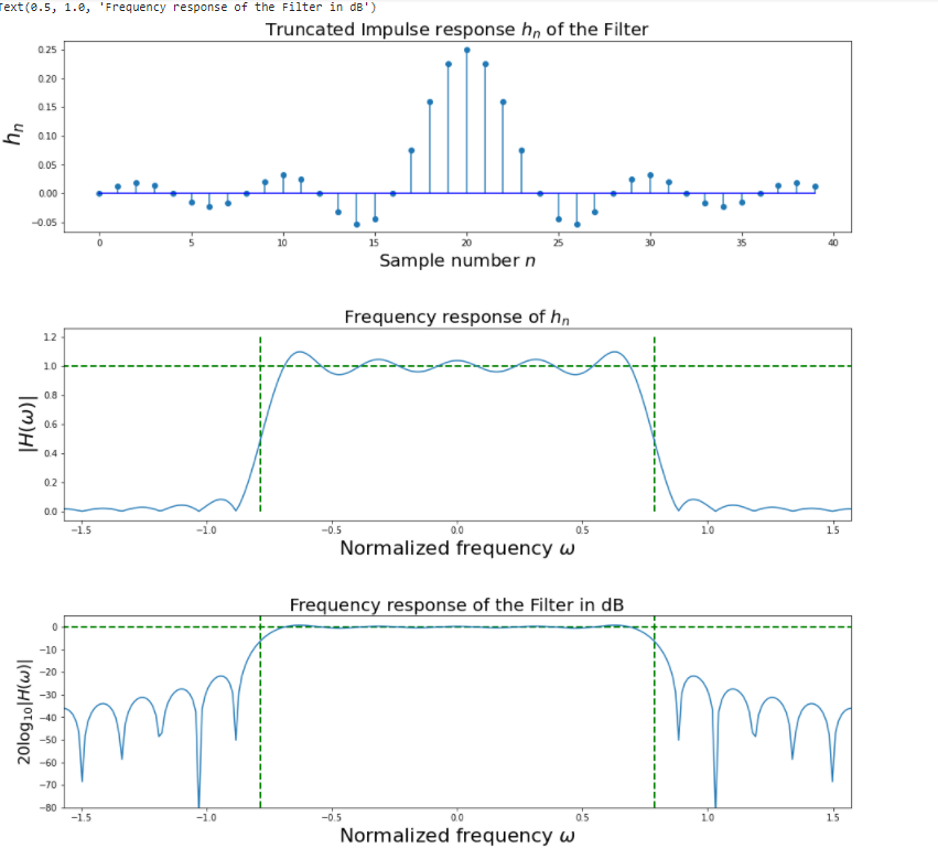
步骤 4：使用矩形窗法绘制滤波器的截断脉冲响应、频率响应、频率响应

蟒蛇3

##Plotting of the results
fig,axs = plt.subplots(3, 1)
fig.set_size_inches((16, 16))
plt.subplots_adjust(hspace = 0.5)
 
#Plot the modified filter coefficients
ax = axs[0]
ax.stem(n + M, h, basefmt =  'b-', use_line_collection = 'True')
ax.set_xlabel("Sample number $n$", fontsize = 20)
ax.set_ylabel(" $h_n$", fontsize = 24)
ax.set_title('Truncated Impulse response $h_n$ of the Filter', fontsize = 20)
 
#Plot the frequency response of the filter in linear units
ax = axs[1]
ax.plot(w-np.pi, abs(np.fft.fftshift(Hh)))
ax.axis(xmax = np.pi/2, xmin = -np.pi/2)
ax.vlines([-wc,wc], 0, 1.2, color = 'g', lw = 2., linestyle = '--',)
ax.hlines(1, -np.pi, np.pi, color = 'g', lw = 2., linestyle = '--',)
ax.set_xlabel(r"Normalized frequency $\omega$",fontsize = 22)
ax.set_ylabel(r"$|H(\omega)| $",fontsize = 22)
ax.set_title('Frequency response of $h_n$ ', fontsize = 20)
 
#Plot the frequency response of the filter in dB
ax=axs[2]
ax.plot(w-np.pi, 20*np.log10(abs(np.fft.fftshift(Hh))))
ax.axis(ymin = -80,xmax = np.pi/2,xmin = -np.pi/2)
ax.vlines([-wc,wc], 10, -80, color = 'g', lw = 2., linestyle = '--',)
ax.hlines(0, -np.pi, np.pi, color = 'g', lw = 2., linestyle = '--',)
ax.set_xlabel(r"Normalized frequency $\omega$",fontsize = 22)
ax.set_ylabel(r"$20\log_{10}|H(\omega)| $",fontsize = 18)
ax.set_title('Frequency response of the Filter in dB', fontsize = 20)

步骤 5：计算幅度、相位响应以获得汉明窗系数

蟒蛇3

#Desired impulse response coefficients of the lowpass filter with cutoff frequency wc
hd=wc/np.pi*np.sinc(wc*(n)/np.pi)### START CODE HERE ### (≈ 1 line of code)
 
#Select the rectangular window coefficients
win =signal.hamming(len(n))### START CODE HERE ### (≈ 1 line of code)
 
#Perform multiplication of desired coefficients and window
#coefficients in time domain
#instead of convolving in frequency domain
h = hd*win### START CODE HERE ### (≈ 1 line of code ## Modified filter coefficients
 
##Compute the frequency response of the modified filter coefficients
w,Hh =signal.freqz(h,1,whole=True,worN=N)### START CODE HERE ### (≈ 1 line of code)     
## get entire frequency domain
 
##Shift the FFT to center for plotting
wx =np.fft.fftfreq(len(w))### START CODE HERE ### (≈ 1 line of code)  

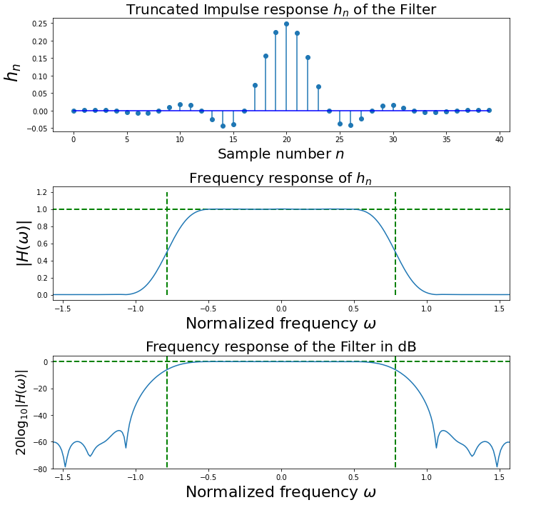
步骤 6：使用汉明窗法绘制滤波器的截断脉冲响应、频率响应、频率响应

蟒蛇3

##Plotting of the results
fig,axs = plt.subplots(3,1)
fig.set_size_inches((10,10))
plt.subplots_adjust(hspace=0.5)
 
#Plot the modified filter coefficients
ax=axs[0]
ax.stem(n+M, h, basefmt='b-', use_line_collection='True')
ax.set_xlabel("Sample number $n$",fontsize=20)
ax.set_ylabel(" $h_n$",fontsize=24)
ax.set_title('Truncated Impulse response $h_n$ of the Filter', fontsize=20)
 
#Plot the frequency response of the filter in linear units
ax=axs[1]
ax.plot(w-np.pi, abs(np.fft.fftshift(Hh)))
ax.axis(xmax=np.pi/2, xmin=-np.pi/2)
ax.vlines([-wc,wc], 0, 1.2, color='g', lw=2., linestyle='--',)
ax.hlines(1, -np.pi, np.pi, color='g', lw=2., linestyle='--',)
ax.set_xlabel(r"Normalized frequency $\omega$",fontsize=22)
ax.set_ylabel(r"$|H(\omega)| $",fontsize=22)
ax.set_title('Frequency response of $h_n$ ', fontsize=20)
 
#Plot the frequency response of the filter in dB
ax=axs[2]
ax.plot(w-np.pi, 20*np.log10(abs(np.fft.fftshift(Hh))))
ax.axis(ymin=-80,xmax=np.pi/2,xmin=-np.pi/2)
ax.vlines([-wc,wc], 10, -80, color='g', lw=2., linestyle='--',)
ax.hlines(0, -np.pi, np.pi, color='g', lw=2., linestyle='--',)
ax.set_xlabel(r"Normalized frequency $\omega$",fontsize=22)
ax.set_ylabel(r"$20\log_{10}|H(\omega)| $",fontsize=18)
ax.set_title('Frequency response of the Filter in dB', fontsize=20)
 
fig.tight_layout()
plt.show()

蟒蛇3

#Desired impulse response coefficients of the lowpass filter with cutoff frequency wc
hd=wc/np.pi*np.sinc(wc*(n)/np.pi)### START CODE HERE ### (≈ 1 line of code)
 
#Select the rectangular window coefficients
win =signal.hamming(len(n))### START CODE HERE ### (≈ 1 line of code)
 
#Perform multiplication of desired coefficients and window
#coefficients in time domain
#instead of convolving in frequency domain
h = hd*win### START CODE HERE ### (≈ 1 line of code ## Modified filter coefficients
 
##Compute the frequency response of the modified filter coefficients
w,Hh =signal.freqz(h,1,whole=True,worN=N)### START CODE HERE ### (≈ 1 line of code)     
## get entire frequency domain
 
##Shift the FFT to center for plotting
wx =np.fft.fftfreq(len(w))### START CODE HERE ### (≈ 1 line of code)