毫升 |信用卡欺诈检测
挑战在于识别欺诈性信用卡交易,以便信用卡公司的客户不会因为他们没有购买的商品而被收取费用。
信用卡欺诈检测涉及的主要挑战是:
- 每天都会处理海量数据,模型构建必须足够快才能及时响应骗局。
- 不平衡数据,即大多数交易(99.8%)不是欺诈性的,这使得检测欺诈性交易变得非常困难
- 数据可用性,因为数据大多是私有的。
- 错误分类的数据可能是另一个主要问题,因为并非每笔欺诈交易都会被捕获和报告。
- 诈骗者对模型使用的自适应技术。
如何应对这些挑战?
- 所使用的模型必须足够简单和快速,以检测异常并将其尽快归类为欺诈交易。
- 不平衡可以通过适当使用一些我们将在下一段中讨论的方法来处理
- 为了保护用户的隐私,可以减少数据的维数。
- 必须采用更可靠的来源来仔细检查数据,至少在训练模型时。
- 我们可以使模型简单且可解释,这样当诈骗者通过一些调整来适应它时,我们就可以启动并运行一个新模型来部署。
在进入代码之前,需要在 jupyter notebook 上工作。如果您的机器上没有安装,您可以使用 Google colab。
您可以从此链接下载数据集
如果链接不起作用,请转到此链接并登录 kaggle 下载数据集。
代码:导入所有必要的库
# import the necessary packages
import numpy as np
import pandas as pd
import matplotlib.pyplot as plt
import seaborn as sns
from matplotlib import gridspec
代码:加载数据
# Load the dataset from the csv file using pandas
# best way is to mount the drive on colab and
# copy the path for the csv file
data = pd.read_csv("credit.csv")
代码:理解数据
# Grab a peek at the data
data.head()

代码:描述数据
# Print the shape of the data
# data = data.sample(frac = 0.1, random_state = 48)
print(data.shape)
print(data.describe())
输出 :
(284807, 31)
                Time            V1  ...         Amount          Class
count  284807.000000  2.848070e+05  ...  284807.000000  284807.000000
mean    94813.859575  3.919560e-15  ...      88.349619       0.001727
std     47488.145955  1.958696e+00  ...     250.120109       0.041527
min         0.000000 -5.640751e+01  ...       0.000000       0.000000
25%     54201.500000 -9.203734e-01  ...       5.600000       0.000000
50%     84692.000000  1.810880e-02  ...      22.000000       0.000000
75%    139320.500000  1.315642e+00  ...      77.165000       0.000000
max    172792.000000  2.454930e+00  ...   25691.160000       1.000000

[8 rows x 31 columns]
代码:数据不平衡
是时候解释我们正在处理的数据了。
# Determine number of fraud cases in dataset
fraud = data[data['Class'] == 1]
valid = data[data['Class'] == 0]
outlierFraction = len(fraud)/float(len(valid))
print(outlierFraction)
print('Fraud Cases: {}'.format(len(data[data['Class'] == 1])))
print('Valid Transactions: {}'.format(len(data[data['Class'] == 0])))
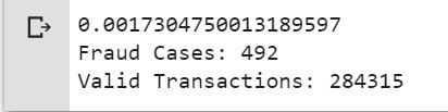
所有交易中只有0.17%的欺诈交易。数据高度不平衡。让我们首先应用我们的模型而不平衡它,如果我们没有得到很好的准确性,那么我们可以找到一种方法来平衡这个数据集。但首先,让我们在没有它的情况下实现模型,并且仅在需要时才平衡数据。
代码:打印欺诈交易的金额详细信息
print(“Amount details of the fraudulent transaction”)
fraud.Amount.describe()
输出 :
Amount details of the fraudulent transaction
count     492.000000
mean      122.211321
std       256.683288
min         0.000000
25%         1.000000
50%         9.250000
75%       105.890000
max      2125.870000
Name: Amount, dtype: float64
代码:打印正常交易的金额详细信息
print(“details of valid transaction”)
valid.Amount.describe()
输出 :
Amount details of valid transaction
count    284315.000000
mean         88.291022
std         250.105092
min           0.000000
25%           5.650000
50%          22.000000
75%          77.050000
max       25691.160000
Name: Amount, dtype: float64
从中我们可以清楚地注意到,欺诈者的平均货币交易更多。这使得这个问题变得至关重要。
代码:绘制相关矩阵
相关矩阵以图形方式让我们了解特征如何相互关联,并可以帮助我们预测与预测最相关的特征是什么。
# Correlation matrix
corrmat = data.corr()
fig = plt.figure(figsize = (12, 9))
sns.heatmap(corrmat, vmax = .8, square = True)
plt.show()

在 HeatMap 中,我们可以清楚地看到大多数特征与其他特征不相关,但有些特征彼此之间存在正相关或负相关。例如, V2和V5与称为Amount的特征高度负相关。我们还看到了与V20和Amount的一些相关性。这使我们对可用的数据有更深入的了解。
代码:分离 X 和 Y 值
将数据划分为输入参数和输出值格式
# dividing the X and the Y from the dataset
X = data.drop(['Class'], axis = 1)
Y = data["Class"]
print(X.shape)
print(Y.shape)
# getting just the values for the sake of processing
# (its a numpy array with no columns)
xData = X.values
yData = Y.values
输出 :
(284807, 30)
(284807, )
训练和测试数据分叉
我们将数据集分为两个主要组。一个用于训练模型,另一个用于测试我们训练好的模型的性能。
# Using Skicit-learn to split data into training and testing sets
from sklearn.model_selection import train_test_split
# Split the data into training and testing sets
xTrain, xTest, yTrain, yTest = train_test_split(
        xData, yData, test_size = 0.2, random_state = 42)
代码:使用 skicit learn 构建随机森林模型
# Building the Random Forest Classifier (RANDOM FOREST)
from sklearn.ensemble import RandomForestClassifier
# random forest model creation
rfc = RandomForestClassifier()
rfc.fit(xTrain, yTrain)
# predictions
yPred = rfc.predict(xTest)
代码:构建各种评估参数
# Evaluating the classifier
# printing every score of the classifier
# scoring in anything
from sklearn.metrics import classification_report, accuracy_score
from sklearn.metrics import precision_score, recall_score
from sklearn.metrics import f1_score, matthews_corrcoef
from sklearn.metrics import confusion_matrix

n_outliers = len(fraud)
n_errors = (yPred != yTest).sum()
print("The model used is Random Forest classifier")

acc = accuracy_score(yTest, yPred)
print("The accuracy is {}".format(acc))

prec = precision_score(yTest, yPred)
print("The precision is {}".format(prec))

rec = recall_score(yTest, yPred)
print("The recall is {}".format(rec))

f1 = f1_score(yTest, yPred)
print("The F1-Score is {}".format(f1))

MCC = matthews_corrcoef(yTest, yPred)
print("The Matthews correlation coefficient is{}".format(MCC))
输出 :
The model used is Random Forest classifier
The accuracy is  0.9995611109160493
The precision is 0.9866666666666667
The recall is 0.7551020408163265
The F1-Score is 0.8554913294797689
The Matthews correlation coefficient is0.8629589216367891
代码:可视化混淆矩阵
# printing the confusion matrix
LABELS = ['Normal', 'Fraud']
conf_matrix = confusion_matrix(yTest, yPred)
plt.figure(figsize =(12, 12))
sns.heatmap(conf_matrix, xticklabels = LABELS,
            yticklabels = LABELS, annot = True, fmt ="d");
plt.title("Confusion matrix")
plt.ylabel('True class')
plt.xlabel('Predicted class')
plt.show()
输出 :

在不处理数据不平衡的情况下与其他算法进行比较。 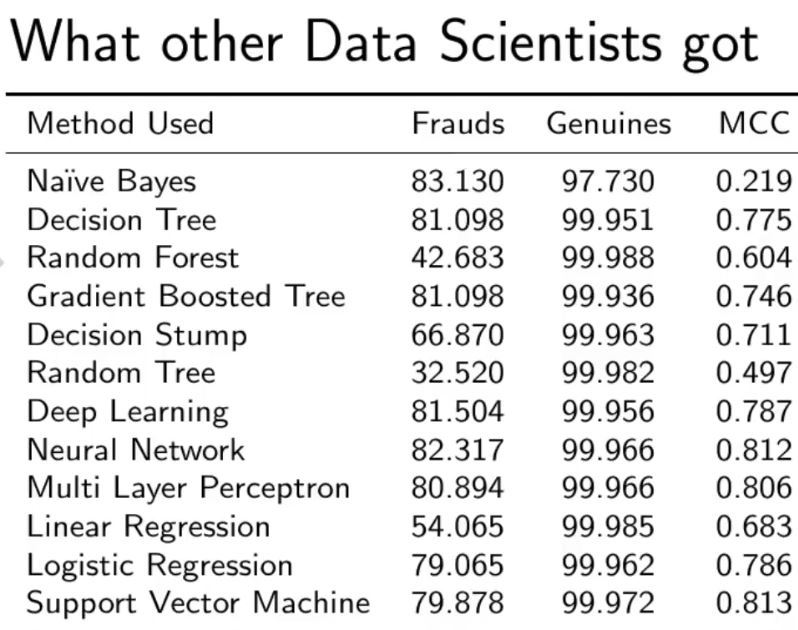
正如您在我们的随机森林模型中看到的那样,即使对于最棘手的部分召回,我们也得到了更好的结果。
在评论中写代码?请使用 ide.geeksforgeeks.org,生成链接并在此处分享链接。