R中矩阵的代数运算
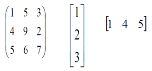
矩阵是行和列中数字的矩形排列。在矩阵中,我们知道行是水平运行的,列是垂直运行的。在 R 中,矩阵是二维的同质数据结构。这些是矩阵的一些示例。
基本代数运算是算术的任何一种传统运算,包括加法、减法、乘法、除法、整数幂和求根。这些运算可以在数字上执行,在这种情况下,它们通常称为算术运算。我们可以对 R 中的矩阵执行更多代数运算。可以对 R 中的矩阵执行的代数运算:
- 对单个矩阵的操作
- 一元运算
- 二元运算
- 线性代数运算
- 矩阵的秩、行列式、转置、逆、迹
- 矩阵的空值
- 矩阵的特征值和特征向量
- 求解线性矩阵方程
对单个矩阵的操作
我们可以使用重载的算术运算运算符对矩阵进行逐元素运算以创建新矩阵。在 +=、-=、*=运算符的情况下,修改现有矩阵。
# R program to demonstrate
# basic operations on a single matrix

# Create a 3x3 matrix
a = matrix(
  c(1, 2, 3, 4, 5, 6, 7, 8, 9),
  nrow = 3,
  ncol = 3,
  byrow = TRUE
)
cat("The 3x3 matrix:\n")
print(a)

# add 1 to every element
cat("Adding 1 to every element:\n")
print(a + 1)

# subtract 3 from each element
cat("Subtracting 3 from each element:\n")
print(a-3)

# multiply each element by 10
cat("Multiplying each element by 10:\n")
print(a * 10)

# square each element
cat("Squaring each element:\n")
print(a ^ 2)

# modify existing matrix
cat("Doubled each element of original matrix:\n")
print(a * 2)
输出:
The 3x3 matrix:
     [, 1] [, 2] [, 3]
[1, ]    1    2    3
[2, ]    4    5    6
[3, ]    7    8    9
Adding 1 to every element:
     [, 1] [, 2] [, 3]
[1, ]    2    3    4
[2, ]    5    6    7
[3, ]    8    9   10
Subtracting 3 from each element:
     [, 1] [, 2] [, 3]
[1, ]   -2   -1    0
[2, ]    1    2    3
[3, ]    4    5    6
Multiplying each element by 10:
     [, 1] [, 2] [, 3]
[1, ]   10   20   30
[2, ]   40   50   60
[3, ]   70   80   90
Squaring each element:
     [, 1] [, 2] [, 3]
[1, ]    1    4    9
[2, ]   16   25   36
[3, ]   49   64   81
Doubled each element of original matrix:
     [, 1] [, 2] [, 3]
[1, ]    2    4    6
[2, ]    8   10   12
[3, ]   14   16   18
一元运算
可以对 R 中的矩阵执行许多一元运算。这包括求和、最小值、最大值等。
# R program to demonstrate
# unary operations on a matrix

# Create a 3x3 matrix
a = matrix(
  c(1, 2, 3, 4, 5, 6, 7, 8, 9),
  nrow = 3,
  ncol = 3,
  byrow = TRUE
)
cat("The 3x3 matrix:\n")
print(a)

# maximum element in the matrix
cat("Largest element is:\n")
print(max(a))

# minimum element in the matrix
cat("Smallest element is:\n")
print(min(a))

# sum of element in the matrix
cat("Sum of elements is:\n")
print(sum(a))
输出:
The 3x3 matrix:
     [, 1] [, 2] [, 3]
[1, ]    1    2    3
[2, ]    4    5    6
[3, ]    7    8    9
Largest element is:
[1] 9
Smallest element is:
[1] 1
Sum of elements is:
[1] 45
二元运算
这些操作按元素应用于矩阵,并创建一个新矩阵。您可以使用所有基本的算术运算运算符,如 +、-、*、/ 等。在 +=、-=、=运算符的情况下,将修改现有矩阵。
# R program to demonstrate
# binary operations on a matrix

# Create a 3x3 matrix
a = matrix(
  c(1, 2, 3, 4, 5, 6, 7, 8, 9),
  nrow = 3,
  ncol = 3,
  byrow = TRUE
)
cat("The 3x3 matrix:\n")
print(a)

# Create another 3x3 matrix
b = matrix(
  c(1, 2, 5, 4, 6, 2, 9, 4, 3),
  nrow = 3,
  ncol = 3,
  byrow = TRUE
)
cat("The another 3x3 matrix:\n")
print(b)

cat("Matrix addition:\n")
print(a + b)

cat("Matrix substraction:\n")
print(a-b)

cat("Matrix element wise multiplication:\n")
print(a * b)

cat("Regular Matrix multiplication:\n")
print(a %*% b)

cat("Matrix elementwise division:\n")
print(a / b)
输出:
The 3x3 matrix:
     [, 1] [, 2] [, 3]
[1, ]    1    2    3
[2, ]    4    5    6
[3, ]    7    8    9
The another 3x3 matrix:
     [, 1] [, 2] [, 3]
[1, ]    1    2    5
[2, ]    4    6    2
[3, ]    9    4    3
Matrix addition:
     [, 1] [, 2] [, 3]
[1, ]    2    4    8
[2, ]    8   11    8
[3, ]   16   12   12
Matrix substraction:
     [, 1] [, 2] [, 3]
[1, ]    0    0   -2
[2, ]    0   -1    4
[3, ]   -2    4    6
Matrix element wise multiplication:
     [, 1] [, 2] [, 3]
[1, ]    1    4   15
[2, ]   16   30   12
[3, ]   63   32   27
Regular Matrix multiplication:
     [, 1] [, 2] [, 3]
[1, ]   36   26   18
[2, ]   78   62   48
[3, ]  120   98   78
Matrix elementwise division:
          [, 1]      [, 2] [, 3]
[1, ] 1.0000000 1.0000000  0.6
[2, ] 1.0000000 0.8333333  3.0
[3, ] 0.7777778 2.0000000  3.0
线性代数运算
可以在 R 中对给定矩阵执行许多线性代数运算。其中一些如下:
- 矩阵的秩、行列式、转置、逆、迹:
# R program to demonstrate
# Linear algebraic operations on a matrix

# Importing required library
library(pracma) # For rank of matrix
library(psych)  # For trace of matrix

# Create a 3x3 matrix
A = matrix(
  c(6, 1, 1, 4, -2, 5, 2, 8, 7),
  nrow = 3,
  ncol = 3,
  byrow = TRUE
)
cat("The 3x3 matrix:\n")
print(A)

# Rank of a matrix
cat("Rank of A:\n")
print(Rank(A))

# Trace of matrix A
cat("Trace of A:\n")
print(tr(A))

# Determinant of a matrix
cat("Determinant of A:\n")
print(det(A))

# Transpose of a matrix
cat("Transpose of A:\n")
print(t(A))

# Inverse of matrix A
cat("Inverse of A:\n")
print(inv(A))
输出:
The 3x3 matrix: [, 1] [, 2] [, 3] [1, ] 6 1 1 [2, ] 4 -2 5 [3, ] 2 8 7 Rank of A: [1] 3 Trace of A: [1] 11 Determinant of A: [1] -306 Transpose of A: [, 1] [, 2] [, 3] [1, ] 6 4 2 [2, ] 1 -2 8 [3, ] 1 5 7 Inverse of A: [, 1] [, 2] [, 3] [1, ] 0.17647059 -0.003267974 -0.02287582 [2, ] 0.05882353 -0.130718954 0.08496732 [3, ] -0.11764706 0.150326797 0.05228758 - 矩阵的空值:
# R program to demonstrate
# nullity of a matrix

# Importing required library
library(pracma)

# Create a 3x3 matrix
a = matrix(
  c(1, 2, 3, 4, 5, 6, 7, 8, 9),
  nrow = 3,
  ncol = 3,
  byrow = TRUE
)
cat("The 3x3 matrix:\n")
print(a)

# No of column
col = ncol(a)

# Rank of matrix
rank = Rank(a)

# Calculating nullity
nullity = col - rank

cat("Nullity of matrix is:\n")
print(nullity)
输出:
The 3x3 matrix: [, 1] [, 2] [, 3] [1, ] 1 2 3 [2, ] 4 5 6 [3, ] 7 8 9 Nullity of matrix is: [1] 1 - 矩阵的特征值和特征向量:
# R program to illustrate
# Eigenvalues and eigenvectors of metrics

# Create a 3x3 matrix
A = matrix(
  c(1, 2, 3, 4, 5, 6, 7, 8, 9),
  nrow = 3,
  ncol = 3,
  byrow = TRUE
)
cat("The 3x3 matrix:\n")
print(A)

# Calculating Eigenvalues and eigenvectors
print(eigen(A))
输出:
The 3x3 matrix: [, 1] [, 2] [, 3] [1, ] 1 2 3 [2, ] 4 5 6 [3, ] 7 8 9 eigen() decomposition $values [1] 1.611684e+01 -1.116844e+00 -1.303678e-15 $vectors [, 1] [, 2] [, 3] [1, ] -0.2319707 -0.78583024 0.4082483 [2, ] -0.5253221 -0.08675134 -0.8164966 [3, ] -0.8186735 0.61232756 0.4082483 - 求解一个线性矩阵方程:
# R program to illustrate
# Solve a linear matrix equation of metrics

# Importing library for applying pseudoinverse
library(MASS)

# Create a 2x2 matrix
A = matrix(
  c(1, 2, 3, 4),
  nrow = 2,
  ncol = 2,
)
cat("A = :\n")
print(A)

# Create another 2x1 matrix
b = matrix(
  c(7, 10),
  nrow = 2,
  ncol = 1,
)
cat("b = :\n")
print(b)

cat("Solution of linear equations:\n")
print(solve(A)%*% b)

cat("Solution of linear equations using pseudoinverse:\n")
print(ginv(A)%*% b)
输出:
A = :
     [, 1] [, 2]
[1, ]    1    3
[2, ]    2    4
b = :
     [, 1]
[1, ]    7
[2, ]   10
Solution of linear equations:
     [, 1]
[1, ]    1
[2, ]    2
Solution of linear equations using pseudoinverse:
     [, 1]
[1, ]    1
[2, ]    2