毫升 |高斯混合的变分贝叶斯推理

先决条件：高斯混合

高斯混合模型假设数据以这样的方式被分成簇，即给定簇中的每个数据点都遵循特定的多变量高斯分布，并且每个簇的多变量高斯分布相互独立。为了在这样的模型中对数据进行聚类，需要计算在给定观察数据的情况下属于给定聚类的数据点的后验概率。用于此目的的一种近似方法是贝叶方法。但是对于大型数据集，边际概率的计算是非常繁琐的。由于只需要为给定点找到最可能的聚类，因此可以使用近似方法，因为它们可以减少机械功。最好的近似方法之一是使用变分贝叶斯推理方法。该方法使用 KL Divergence 和 Mean-Field Approximation 的概念。

以下步骤将演示如何使用 Sklearn 在高斯混合模型中实现变分贝叶斯推理。使用的数据是可以从 Kaggle 下载的信用卡数据。

第 1 步：导入所需的库

import numpy as np
import pandas as pd
import matplotlib.pyplot as plt
from sklearn.mixture import BayesianGaussianMixture
from sklearn.preprocessing import normalize, StandardScaler
from sklearn.decomposition import PCA

第 2 步：加载和清理数据

# Changing the working location to the location of the data
cd "C:\Users\Dev\Desktop\Kaggle\Credit_Card"
  
# Loading the Data
X = pd.read_csv('CC_GENERAL.csv')
  
# Dropping the CUST_ID column from the data
X = X.drop('CUST_ID', axis = 1)
  
# Handling the missing values
X.fillna(method ='ffill', inplace = True)
  
X.head()

第 3 步：预处理数据

# Scaling the data to bring all the attributes to a comparable level
scaler = StandardScaler()
X_scaled = scaler.fit_transform(X)
  
# Normalizing the data so that the data
# approximately follows a Gaussian distribution
X_normalized = normalize(X_scaled)
  
# Converting the numpy array into a pandas DataFrame
X_normalized = pd.DataFrame(X_normalized)
  
# Renaming the columns
X_normalized.columns = X.columns
  
X_normalized.head()

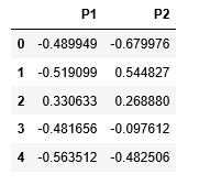
第 4 步：降低数据的维度以使其可视化

# Reducing the dimensions of the data
pca = PCA(n_components = 2)
X_principal = pca.fit_transform(X_normalized)
  
# Converting the reduced data into a pandas dataframe
X_principal = pd.DataFrame(X_principal)
  
# Renaming the columns
X_principal.columns = ['P1', 'P2']
  
X_principal.head()

贝叶斯高斯混合类的主要两个参数是n_components和covariance_type 。

n_components：它确定给定数据中的最大聚类数。
covariance_type：它描述了要使用的协方差参数的类型。

您可以在其文档中阅读所有其他属性。

在下面给出的步骤中，参数 n_components 将固定为 5，而参数 covariance_type 将针对所有可能的值进行更改，以可视化该参数对聚类的影响。

第 5 步：为不同的 covariance_type 值构建聚类模型并可视化结果

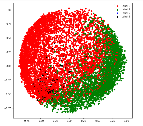
a) covariance_type = 'full'

# Building and training the model
vbgm_model_full = BayesianGaussianMixture(n_components = 5, covariance_type ='full')
vbgm_model_full.fit(X_normalized)
  
# Storing the labels
labels_full = vbgm_model_full.predict(X)
print(set(labels_full))

colours = {}
colours[0] = 'r'
colours[1] = 'g'
colours[2] = 'b'
colours[3] = 'k'
  
# Building the colour vector for each data point
cvec = [colours[label] for label in labels_full]
  
# Defining the scatter plot for each colour
r = plt.scatter(X_principal['P1'], X_principal['P2'], color ='r');
g = plt.scatter(X_principal['P1'], X_principal['P2'], color ='g');
b = plt.scatter(X_principal['P1'], X_principal['P2'], color ='b');
k = plt.scatter(X_principal['P1'], X_principal['P2'], color ='k');
  
# Plotting the clustered data
plt.figure(figsize =(9, 9))
plt.scatter(X_principal['P1'], X_principal['P2'], c = cvec)
plt.legend((r, g, b, k), ('Label 0', 'Label 1', 'Label 2', 'Label 3'))
plt.show()

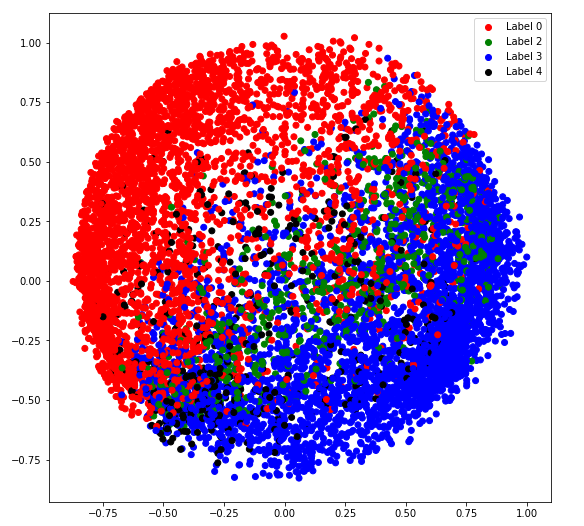
b) covariance_type = '并列'

# Building and training the model
vbgm_model_tied = BayesianGaussianMixture(n_components = 5, covariance_type ='tied')
vbgm_model_tied.fit(X_normalized)
  
# Storing the labels
labels_tied = vbgm_model_tied.predict(X)
print(set(labels_tied))

colours = {}
colours[0] = 'r'
colours[2] = 'g'
colours[3] = 'b'
colours[4] = 'k'
  
# Building the colour vector for each data point
cvec = [colours[label] for label in labels_tied]
  
# Defining the scatter plot for each colour
r = plt.scatter(X_principal['P1'], X_principal['P2'], color ='r');
g = plt.scatter(X_principal['P1'], X_principal['P2'], color ='g');
b = plt.scatter(X_principal['P1'], X_principal['P2'], color ='b');
k = plt.scatter(X_principal['P1'], X_principal['P2'], color ='k');
  
# Plotting the clustered data
plt.figure(figsize =(9, 9))
plt.scatter(X_principal['P1'], X_principal['P2'], c = cvec)
plt.legend((r, g, b, k), ('Label 0', 'Label 2', 'Label 3', 'Label 4'))
plt.show()

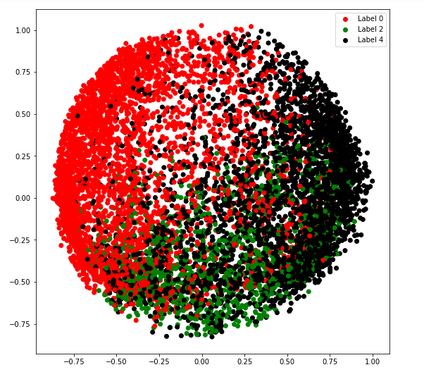
c) covariance_type = '诊断'

# Building and training the model
vbgm_model_diag = BayesianGaussianMixture(n_components = 5, covariance_type ='diag')
vbgm_model_diag.fit(X_normalized)
  
# Storing the labels
labels_diag = vbgm_model_diag.predict(X)
print(set(labels_diag))

colours = {}
colours[0] = 'r'
colours[2] = 'g'
colours[4] = 'k'
  
# Building the colour vector for each data point
cvec = [colours[label] for label in labels_diag]
  
# Defining the scatter plot for each colour
r = plt.scatter(X_principal['P1'], X_principal['P2'], color ='r');
g = plt.scatter(X_principal['P1'], X_principal['P2'], color ='g');
k = plt.scatter(X_principal['P1'], X_principal['P2'], color ='k');
  
# Plotting the clustered data
plt.figure(figsize =(9, 9))
plt.scatter(X_principal['P1'], X_principal['P2'], c = cvec)
plt.legend((r, g, k), ('Label 0', 'Label 2', 'Label 4'))
plt.show()

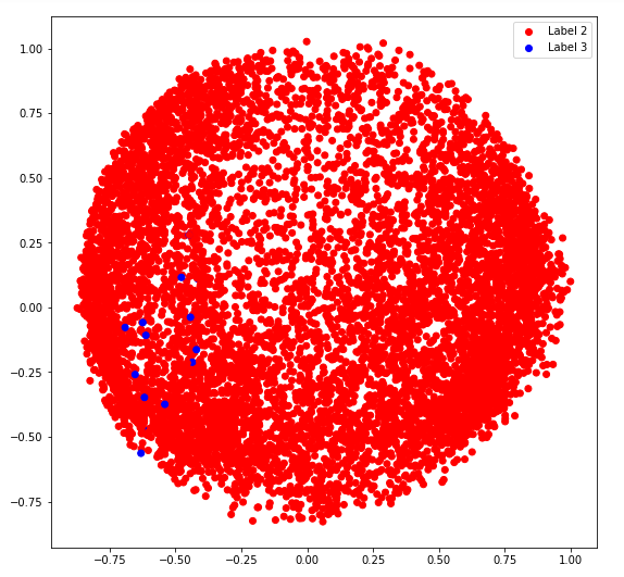
d) covariance_type = '球形'

# Building and training the model
vbgm_model_spherical = BayesianGaussianMixture(n_components = 5,
                                              covariance_type ='spherical')
vbgm_model_spherical.fit(X_normalized)
  
# Storing the labels
labels_spherical = vbgm_model_spherical.predict(X)
print(set(labels_spherical))

colours = {}
colours[2] = 'r'
colours[3] = 'b'
  
# Building the colour vector for each data point
cvec = [colours[label] for label in labels_spherical]
  
# Defining the scatter plot for each colour
r = plt.scatter(X_principal['P1'], X_principal['P2'], color ='r');
b = plt.scatter(X_principal['P1'], X_principal['P2'], color ='b');
  
# Plotting the clustered data
plt.figure(figsize =(9, 9))
plt.scatter(X_principal['P1'], X_principal['P2'], c = cvec)
plt.legend((r, b), ('Label 2', 'Label 3'))
plt.show()