R 编程中的正则化

正则化是一种回归技术，可将系数估计缩小或正则化或约束到 0（或零）。在这种技术中，为了降低给定模型的自由度，对模型的各种参数添加了惩罚。正则化的概念大致可以分为：

• 岭回归
• 套索回归
• 弹性网络回归

R中的实现

在 R 语言中，要执行正则化，我们需要在开始处理它们之前安装一些包。所需的软件包是

• 用于岭回归和套索回归的glmnet包
• 用于数据清理的dplyr包
• psych包，用于执行或计算矩阵的跟踪函数
• 插入符号包

要安装这些包，我们必须使用 R 控制台中的install.packages() 。成功安装包后，我们使用library()命令将这些包包含在我们的 R 脚本中。为了实现正则化回归技术，我们需要遵循三种正则化技术中的任何一种。

岭回归

岭回归是线性回归的修改版本，也称为L2 正则化。与线性回归不同，损失函数被修改以最小化模型的复杂性，这是通过添加一些惩罚参数来完成的，该惩罚参数相当于系数值或大小的平方。基本上，要在 R 中实现岭回归，我们将使用“ glmnet ”包。 cv.glmnet()函数将用于确定岭回归。

例子：

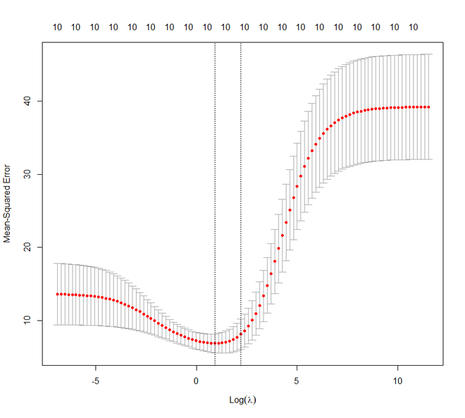
在这个例子中，我们将在mtcars数据集上实现岭回归技术，以获得更好的说明。我们的任务是根据汽车的其他特性预测每加仑行驶里程。我们将使用set.seed()函数来设置种子以实现可重复性。我们将通过三种方式设置 lambda 的值：

• 通过执行 10 折交叉验证
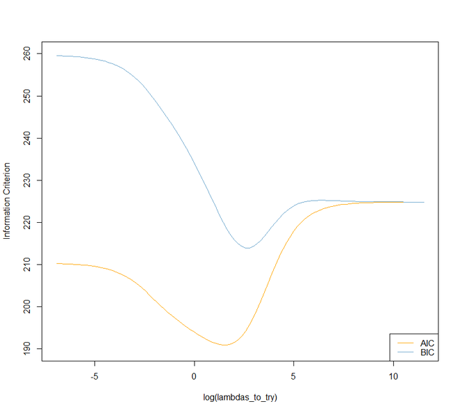
• 基于得到的信息
• 基于这两个标准的最佳 lambda

R

# Regularization
# Ridge Regression in R
# Load libraries, get data & set
# seed for reproducibility 
set.seed(123)    
library(glmnet)  
library(dplyr)   
library(psych)
  
data("mtcars")
# Center y, X will be standardized 
# in the modelling function
y <- mtcars %>% select(mpg) %>% 
            scale(center = TRUE, scale = FALSE) %>% 
            as.matrix()
X <- mtcars %>% select(-mpg) %>% as.matrix()
  
# Perform 10-fold cross-validation to select lambda
lambdas_to_try <- 10^seq(-3, 5, length.out = 100)
  
# Setting alpha = 0 implements ridge regression
ridge_cv <- cv.glmnet(X, y, alpha = 0, 
                      lambda = lambdas_to_try,
                      standardize = TRUE, nfolds = 10)
  
# Plot cross-validation results
plot(ridge_cv)
  
# Best cross-validated lambda
lambda_cv <- ridge_cv$lambda.min
  
# Fit final model, get its sum of squared
# residuals and multiple R-squared
model_cv <- glmnet(X, y, alpha = 0, lambda = lambda_cv,
                   standardize = TRUE)
y_hat_cv <- predict(model_cv, X)
ssr_cv <- t(y - y_hat_cv) %*% (y - y_hat_cv)
rsq_ridge_cv <- cor(y, y_hat_cv)^2
  
# selecting lambda based on the information
X_scaled <- scale(X)
aic <- c()
bic <- c()
for (lambda in seq(lambdas_to_try)) 
{
  # Run model
  model <- glmnet(X, y, alpha = 0,
                  lambda = lambdas_to_try[lambda], 
                  standardize = TRUE)
    
  # Extract coefficients and residuals (remove first 
  # row for the intercept)
  betas <- as.vector((as.matrix(coef(model))[-1, ]))
  resid <- y - (X_scaled %*% betas)
    
  # Compute hat-matrix and degrees of freedom
  ld <- lambdas_to_try[lambda] * diag(ncol(X_scaled))
  H <- X_scaled %*% solve(t(X_scaled) %*% X_scaled + ld) 
                                           %*% t(X_scaled)
  df <- tr(H)
    
  # Compute information criteria
  aic[lambda] <- nrow(X_scaled) * log(t(resid) %*% resid) 
                                                   + 2 * df
  bic[lambda] <- nrow(X_scaled) * log(t(resid) %*% resid)
                           + 2 * df * log(nrow(X_scaled))
}
  
# Plot information criteria against tried values of lambdas
plot(log(lambdas_to_try), aic, col = "orange", type = "l",
     ylim = c(190, 260), ylab = "Information Criterion")
lines(log(lambdas_to_try), bic, col = "skyblue3")
legend("bottomright", lwd = 1, col = c("orange", "skyblue3"), 
       legend = c("AIC", "BIC"))
  
# Optimal lambdas according to both criteria
lambda_aic <- lambdas_to_try[which.min(aic)]
lambda_bic <- lambdas_to_try[which.min(bic)]
  
# Fit final models, get their sum of 
# squared residuals and multiple R-squared
model_aic <- glmnet(X, y, alpha = 0, lambda = lambda_aic, 
                    standardize = TRUE)
y_hat_aic <- predict(model_aic, X)
ssr_aic <- t(y - y_hat_aic) %*% (y - y_hat_aic)
rsq_ridge_aic <- cor(y, y_hat_aic)^2
  
model_bic <- glmnet(X, y, alpha = 0, lambda = lambda_bic, 
                    standardize = TRUE)
y_hat_bic <- predict(model_bic, X)
ssr_bic <- t(y - y_hat_bic) %*% (y - y_hat_bic)
rsq_ridge_bic <- cor(y, y_hat_bic)^2
  
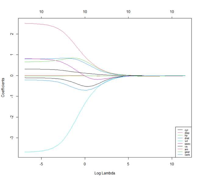
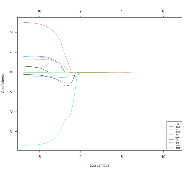
# The higher the lambda, the more the 
# coefficients are shrinked towards zero.
res <- glmnet(X, y, alpha = 0, lambda = lambdas_to_try,
              standardize = FALSE)
plot(res, xvar = "lambda")
legend("bottomright", lwd = 1, col = 1:6, 
       legend = colnames(X), cex = .7)

输出：

套索回归

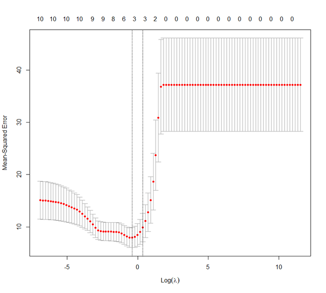
前进到Lasso 回归。它也被称为L1 回归、选择算子和最小绝对收缩。它也是线性回归的修改版本，其中再次修改了损失函数以最小化模型的复杂性。这是通过限制模型系数的绝对值的总和来完成的。在 R 中，我们可以使用与岭回归相同的“ glmnet ”包来实现套索回归。

例子：

在此示例中，我们再次使用mtcars数据集。在这里，我们还将像前面的示例一样设置 lambda 值。

R

# Regularization
# Lasso Regression
# Load libraries, get data & set 
# seed for reproducibility 
set.seed(123)   
library(glmnet)  
library(dplyr)   
library(psych)   
  
data("mtcars")
# Center y, X will be standardized in the modelling function
y <- mtcars %>% select(mpg) %>% scale(center = TRUE, 
                                      scale = FALSE) %>% 
                                      as.matrix()
X <- mtcars %>% select(-mpg) %>% as.matrix()
  
  
# Perform 10-fold cross-validation to select lambda 
lambdas_to_try <- 10^seq(-3, 5, length.out = 100)
  
# Setting alpha = 1 implements lasso regression
lasso_cv <- cv.glmnet(X, y, alpha = 1, 
                      lambda = lambdas_to_try,
                      standardize = TRUE, nfolds = 10)
  
# Plot cross-validation results
plot(lasso_cv)
  
# Best cross-validated lambda
lambda_cv <- lasso_cv$lambda.min
  
# Fit final model, get its sum of squared 
# residuals and multiple R-squared
model_cv <- glmnet(X, y, alpha = 1, lambda = lambda_cv, 
                   standardize = TRUE)
y_hat_cv <- predict(model_cv, X)
ssr_cv <- t(y - y_hat_cv) %*% (y - y_hat_cv)
rsq_lasso_cv <- cor(y, y_hat_cv)^2
  
# The higher the lambda, the more the 
# coefficients are shrinked towards zero.
res <- glmnet(X, y, alpha = 1, lambda = lambdas_to_try,
              standardize = FALSE)
plot(res, xvar = "lambda")
legend("bottomright", lwd = 1, col = 1:6, 
       legend = colnames(X), cex = .7)

输出：

如果我们比较 Lasso 和 Ridge 回归技术，我们会注意到这两种技术或多或少是相同的。但是它们之间几乎没有什么不同的特征。

• 与 Ridge 不同，Lasso 可以将其某些参数设置为零。
• 在岭中，相关的预测变量的系数是相似的。而在套索中，只有一个预测系数较大，其余的趋于零。
• 如果存在许多具有相同值的巨大或大参数，则 Ridge 效果很好。如果仅存在少量确定或重要的参数并且其余参数趋于零，则套索可以很好地工作。

弹性网络回归

我们现在将继续讨论弹性网络回归。弹性网络回归可以说是套索和岭回归的凸组合。我们甚至可以在这里使用glmnet包。但是现在我们将看到如何使用包插入符号来实现弹性网络回归。

例子：

R

# Regularization
# Elastic Net Regression
library(caret)
  
# Set training control
train_control <- trainControl(method = "repeatedcv",
                              number = 5,
                              repeats = 5,
                              search = "random",
                              verboseIter = TRUE)
  
# Train the model
elastic_net_model <- train(mpg ~ .,
                           data = cbind(y, X),
                           method = "glmnet",
                           preProcess = c("center", "scale"),
                           tuneLength = 25,
                           trControl = train_control)
  
# Check multiple R-squared
y_hat_enet <- predict(elastic_net_model, X)
rsq_enet <- cor(y, y_hat_enet)^2
  
print(y_hat_enet)
print(rsq_enet)

输出：

> print(y_hat_enet)
          Mazda RX4       Mazda RX4 Wag          Datsun 710      Hornet 4 Drive   Hornet Sportabout             Valiant 
         2.13185747          1.76214273          6.07598463          0.50410531         -3.15668592          0.08734383 
         Duster 360           Merc 240D            Merc 230            Merc 280           Merc 280C          Merc 450SE 
        -5.23690809          2.82725225          2.85570982         -0.19421572         -0.16329225         -4.37306992 
         Merc 450SL         Merc 450SLC  Cadillac Fleetwood Lincoln Continental   Chrysler Imperial            Fiat 128 
        -3.83132657         -3.88886320         -8.00151118         -8.29125966         -8.08243188          6.98344302 
        Honda Civic      Toyota Corolla       Toyota Corona    Dodge Challenger         AMC Javelin          Camaro Z28 
         8.30013895          7.74742320          3.93737683         -3.13404917         -2.56900144         -5.17326892 
   Pontiac Firebird           Fiat X1-9       Porsche 914-2        Lotus Europa      Ford Pantera L        Ferrari Dino 
        -4.02993835          7.36692700          5.87750517          6.69642869         -2.02711333          0.06597788 
      Maserati Bora          Volvo 142E 
        -5.90030273          4.83362156 
> print(rsq_enet)
         [,1]
mpg 0.8485501